Chapter 9 Solutions
Contributed by Protensia Hadunka and Rachel Richardson 2017
9.1
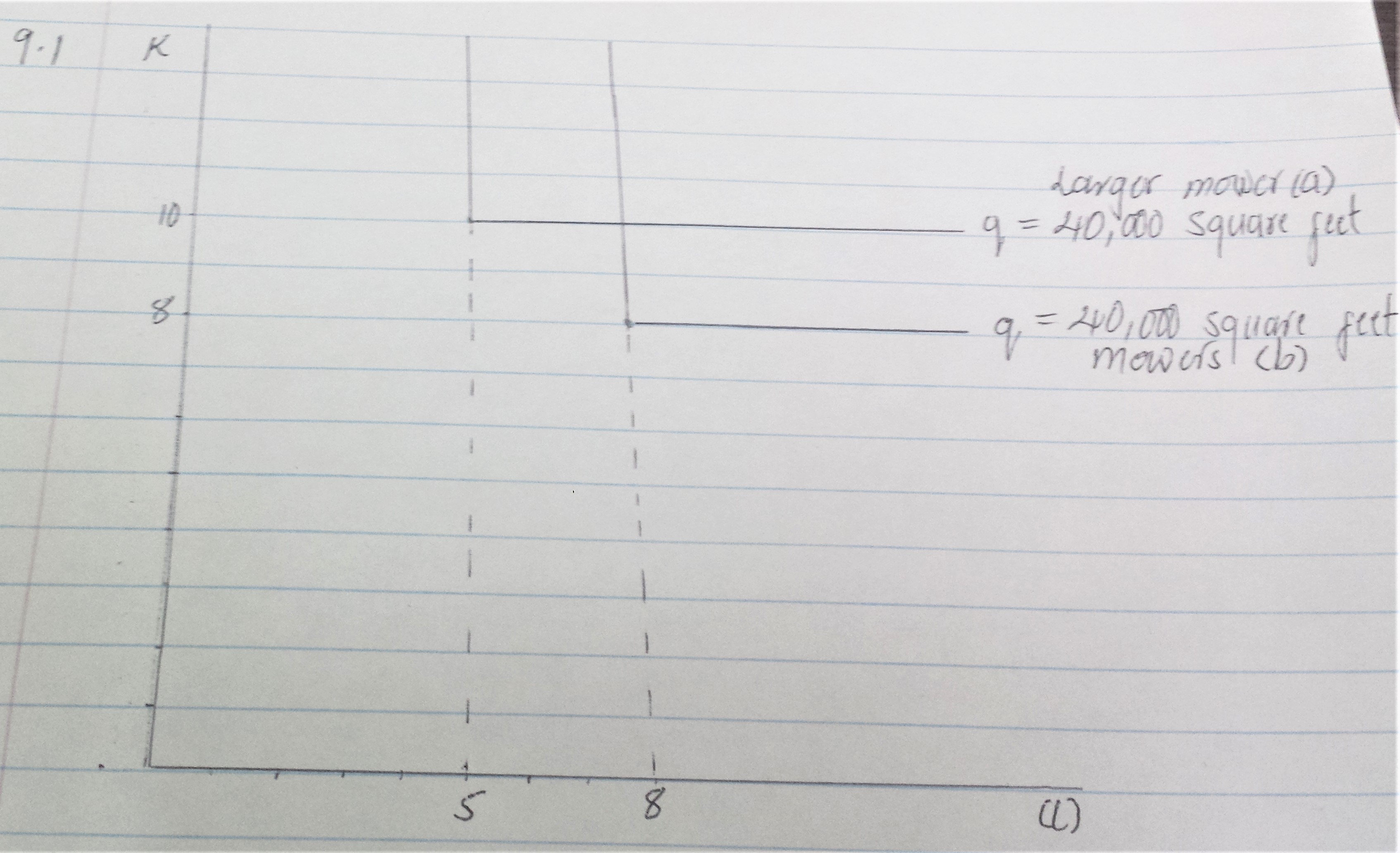
Figure 1.
\(q=40,000\) sq ft requires 5 hours of labor and 10 units of capital (# of 24 mowers)
\(q=40,000\) sq ft requires 8 hours of labor and 8 units of capital (# of 24 mowers)
\(q=20,000\) sq ft requires 2.5 hours of labor and 5 units of capital (# of 24 mowers)
\(q=40,000\) sq ft requires 4 hours of labor and 4 units of capital (# of 24 mowers)
Total 40,000 6.5 hours of labor and 9 units of capital
\(q=30,000\) sq ft requires 3.75 hours of labor and 7.5 units of capital large
\(q=10,000\) sq ft requires 2 hours of labor and 2 units of capital large
Total \(q=40,000\) sq ft 5.75 hours of labor and 9.5 units of capital
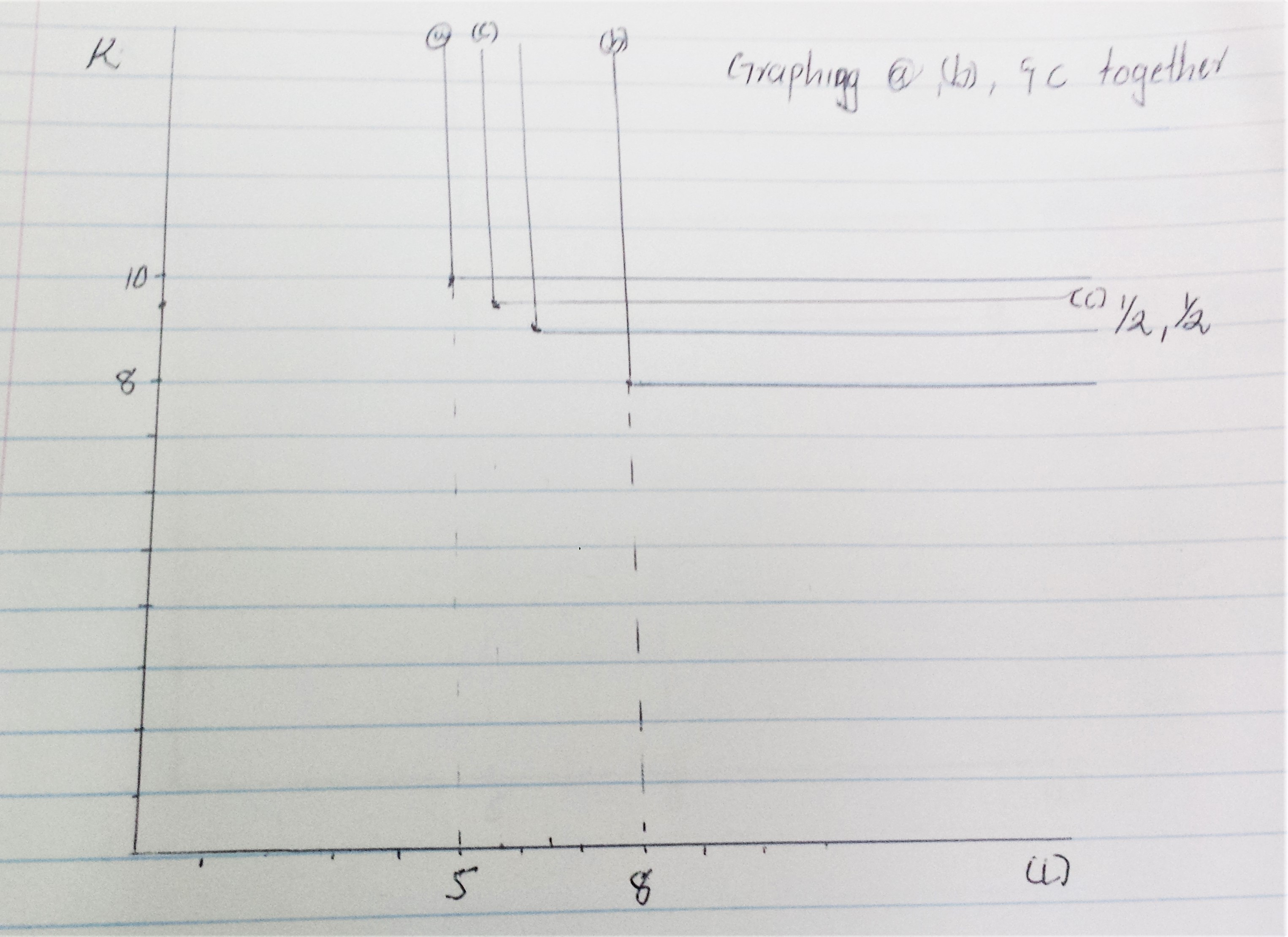
Figure 2.
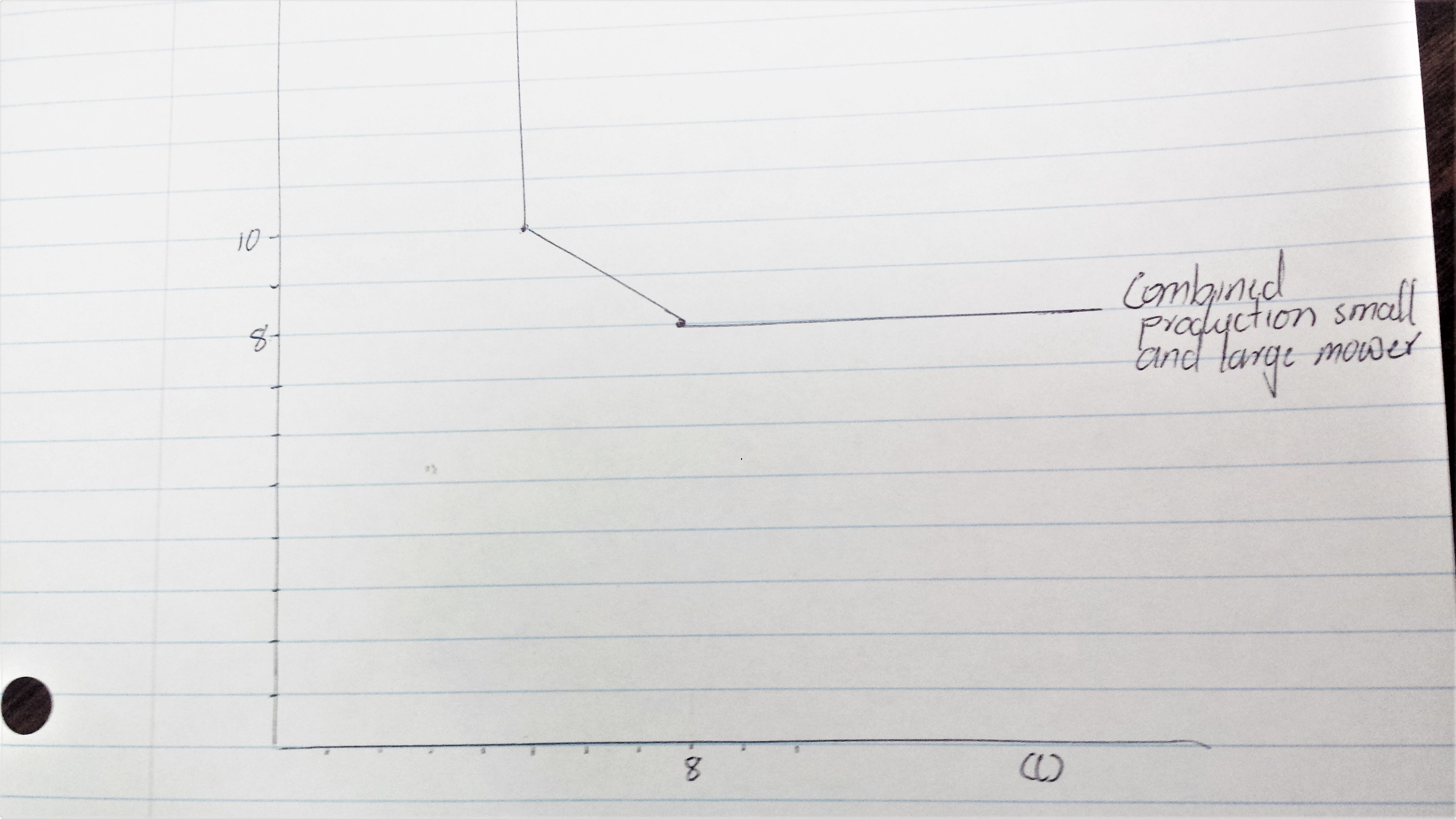
Figure 3.
By varying the proportion mowed with the large mower and small mower, the combined isoquant includes the chord connecting the two vertices of the original isoquant.
9.3
Sam Malone is considering renovating the bar stools at Cheers. The production function for new bar stools is given by,
\[q=0.1k^{0.2}t^{0.8}\]
where q is the number of bar stools produced during the renovation week, k represents the number of hours of bar stool lathes used during the week, and l represents the number of worker hours employed during the period. Sam would like to provide 10 new bar stools, and he has allocated a budget of \(10,000\) for the project Sam reasons that because bar stool lathes and skilled bar stool workers both cost the same amount (\(50\) per hours), he might as well hire these two inputs in equal amounts. If Sam proceeds in this way, how much of each input will he hire and how much will the renovation project cost?
\[q=10\] \[k=l\]\[q=0.1k^{0.2}k^{0.8} = 0.1k\] \[10=0.1k\]\[k=100\]\[k=l=100\] \[Cost=50k+50l\]\[Cost=10,000\]
\[MP_l=\frac{dq}{dl}=(0.1k^{0.2})(0.8l^{-0.2})\]\[MP_k=\frac{dq}{dk}=(0.1)(0.2k^{-0.8})(l^{0.8})\] \[MP_l=MP_k\]\[(0.1k^{-0.2})(0.8l^{0.2})=(0.1)(0.2k^{-0.8})(l^{0.8})\]\[k=\frac{0.2}{0.8}l\] Plug k back into q \[q=0.1[\frac{0.2}{0.8}l]^{0.2}l^{0.8}\] Solve for 10 stools q=10 \[10=0.1[\frac{0.2}{0.8}l]^{0.2}l^{0.8}\]\[10=(0.1)[\frac{0.2}{0.8}]^{0.2}l^{0.2}l^{0.8}\]\[100=[\frac{0.2}{0.8}]^{0.2}l\]\[100*[\frac{0.8}{0.2}]^{0.2}=l\]\[l=131.95\] Solve for k \[k=\frac{0.2}{0.8}*(131.95)\]\[k=32.9875\] \[Cost=(50)(32.9875)+(50)(131.95)\]\[Cost=8,246.875\]
c)\[Cost=10,000-8,246.875=$1,753.125\] Use 1,753.125 for new budget and set equal to cost equation \[k=\frac{0.2}{0.8}l\] \[$1,753.125=(50)(\frac{0.2}{0.8}l)+(50)(l)\] At 1,753.125 \[l=28.0496\]\[k=7.0124\] \[q=(0.1)(7.0124)^{0.2}*(28.0496)^{0.8}\]\[q=2.126\] Sam can afford to produce 2 more stools
d)It depends if Carla’s unhappiness serving extra customers incurs additional costs for the bar.
9.4
- Allocate labor so that the MPs are equal at each site, otherwise you would set more output by adjusting.
\[MP_{l1}=MP_{l2}\] \[5l_1^{-0.5}=25-l_2^{-0.5}\] \[l_1=5l_2^{-2}\] \[l_1=\frac{l_2}{25}\] \[l_1=[5l_2^{-0.5}]^{\frac{-1}{0.5}}\] b) \[q=10l_1^{0.5}+50l_2^{0.5}\] \[q=10[\frac{l_2}{25}]^{0.5}+50l_2^{0.5}\] \[q=2l_2^{0.5}+50l_2^{0.5}\] \[q=l_2^{0.5}\] \[q=52[\frac{25}{26}l]^{0.5}\] To show how why the equation above as it is,follow the steps below: \[l_1+l_2=l\] \[\frac{l_2}{25}+l_2=l\] \[\frac{26}{25}l_2=l\] \[l_2=\frac{25}{26}l\]
\[q=\frac{52.5}{\sqrt{26}}l^{0.5}\]
9.7 Production function generalized from Q9.3
\[q=\beta_0+\beta_1\sqrt{kl}+\beta_2k+\beta_3l\]
CRTS
\[q=f(tk, tl)=tf(k,l)\]\[f(tk,tl)=\beta_0+\beta_1\sqrt{(tk)(tl)}+\beta_2(tk)+\beta_3(tl)\]\[=\beta_0+t\beta_1\sqrt{kl}+t\beta_2k+t\beta_3l\]\[=tf(k,l)\] if and only if \[\beta_0=0\] b) \[MP_l=\frac{1}{2}\beta_1k^{\frac{1}{2}}l^{\frac{-1}{2}}+\beta_3\]\[MP_k=\frac{1}{2}\beta_1k^{\frac{-1}{2}}l^{\frac{1}{2}}+\beta_2\] MPl is diminishing \[\frac{dMP_l}{dl}=\frac{-1}{4}\beta_1k^{\frac{1}{2}}l^{\frac{-3}{2}}<0\] MPk also diminishing \[\frac{dMP_k}{dk}=\frac{-1}{4}\beta_1k^{\frac{-3}{2}}l^{\frac{1}{2}}<0\] Homogeneous degree 0 if \[f(\alpha*x)=\alpha^0f(x)\]1 if \[f(\alpha*x)=\alpha^1f(x)\] until n if \[f(\alpha*x)=\alpha^nf(x)\] To show marginal productivities are homogeneous of degree 0 need to show \[MP_l(\alpha{k},\alpha{l})=\alpha^0MP_l(k,l)\] \[MP_l(\alpha{k},\alpha{l})=\frac{1}{2}\beta_1(\alpha{k})^{\frac{1}{2}}(\alpha{l})^\frac{-1}{2}+\beta_3\]\[=\frac{1}{2}\beta_1\alpha^\frac{1}{2}\alpha^\frac{-1}{2}k^\frac{1}{2}l^\frac{-1}{2}+\beta_3\]\[=\frac{1}{2}\beta_1k^\frac{1}{2}l^\frac{-1}{2}+\beta_3\]\[=\alpha^{0}MP_l(k,l)\] MPl is homogeneous for degree 0 Similar for MPk
- \[\sigma=\frac{\Delta(\frac{k}{l})}{\Delta(RTS)}\] *percent change Note footnote 6 on p305 for the CRTS case: \[\sigma=\frac{f_k*f_l}{f*f_{kl}}\]We have fk & fl from part b) \[f_{kl}=\frac{df_k}{dl}=\frac{d}{dl}(\frac{1}{2}\beta_1k^{\frac{-1}{2}}l^{\frac{1}{2}}+\beta_2)\]\[=\frac{1}{4}\beta_1k^\frac{-1}{2}l^\frac{-1}{2}\]\[\sigma=\frac{f_k*f_l}{f*f_{kl}}\]
\[=\frac{[\frac{1}{2}\beta_1k^\frac{-1}{2}l^\frac{1}{2}+\beta_2][\frac{1}{2}\beta_1k^\frac{1}{2}l^\frac{1}{2}+\beta_3]}{[\beta_1\sqrt{kl}+\beta_2k+\beta_3l][\frac{1}{4}\beta_1k^\frac{-1}{2}l^\frac{-1}{2}]}\] If \(B_2=B_3=0\)
\[=\frac{[\frac{1}{2}\beta_1k^\frac{-1}{2}l^\frac{1}{2}][\frac{1}{2}\beta_1k^\frac{1}{2}l^\frac{1}{2}]}{[\beta_1\sqrt{kl}][\frac{1}{4}\beta_1k^\frac{-1}{2}l^\frac{-1}{2}]}\]
\[=\frac{\beta_1^2l^\frac{1}{2}k^\frac{1}{2}}{[\beta_1\sqrt{kl}][\beta_1]}=1\] If B1=0 \[\sigma=\frac{[\beta_2][\beta_3]}{[\beta_2k+\beta_3l]*0}=\infty\]