Chapter 3 Solutions

3.1

$U(x,y) = 3x+y$

\[\begin{align*} U_1 & = 3x+y \\ y & = U_1 - 3x \\ \end{align*}\]

Then using $MRS = - \left. \frac{\partial y}{\partial x} \right|_{U = constant}$

and we have $MRS = -(-3) = 3$, which is a constant and not decreasing.

$U(x,y) = \sqrt{xy}$

Since utility is un affected by a monotonic increasing transformation, we can square it and evaluate $U(x,y) = xy$ instead since the math will be a little easier.

\[\begin{align*} U_1 & = xy \\ y & = \frac{U_1}{x} \\ \end{align*}\]

Then the $MRS = -\frac{-U_1}{x^2} = \frac{U_1}{x^2}$.

Since $MRS$ clearly decreases as $x$ increases, the indifference curves are convex.

$U(x,y) = \sqrt{x} + y$

then $y = U_1 - \sqrt{x}$ and the $MRS = -(-\frac{1}{2}x^{-\frac{1}{2}}) = \frac{1}{2\sqrt{x}}$.

Clearly this $MRS$ decreases with $x$ so yes these indifference curves are convex.

$U(x,y) = \sqrt{x^2 - y^2}$

Then,

\[\begin{align*} U_1 & = \sqrt{x^2 - y^2}\\ U^2_1 & = x^2 - y^2 \\ y^2 & = x^2 - U^2_1 \\ y & = \sqrt{x^2 - U^2_1} \end{align*}\]

And then finding the $MRS$,

\[\begin{align*} MRS & = - \frac{x}{\sqrt{(x^2 - U^2_1)}} \end{align*}\]

Yes, these indifference curves decrease as x increases, but this is a tricky question because this is not a proper utility curve to begin with.

$U(x,y) = \frac{xy}{x+y}$

\[\begin{align*} U_0 &= \frac{xy}{x+y} \\ U_0(x+y) &= xy \\ U_0x &= xy - U_0y \\ U_0x &= y(x-U_0) \\ y &= \frac{U_0x}{x-U_0} \end{align*}\]

So,

\[\begin{align*} MRS &= -\frac{dy}{dx}\biggr\rvert_{U=U_0} \\ &= -\left( \frac{U_0(x-U_0) - U_0x}{(x-U_0)^2} \right) \\ &= \frac{U_0^2}{(x-U_0)^2} \end{align*}\]

Is the MRS everywhere decreasing?

\[\frac{\partial MRS}{\partial x} = -2U_0(x-U_0)^{-3} < 0\]

for all $x>0$. So yes, the function is quasi-concave.

To check out these and other indifference curves see desmos.com/calculator

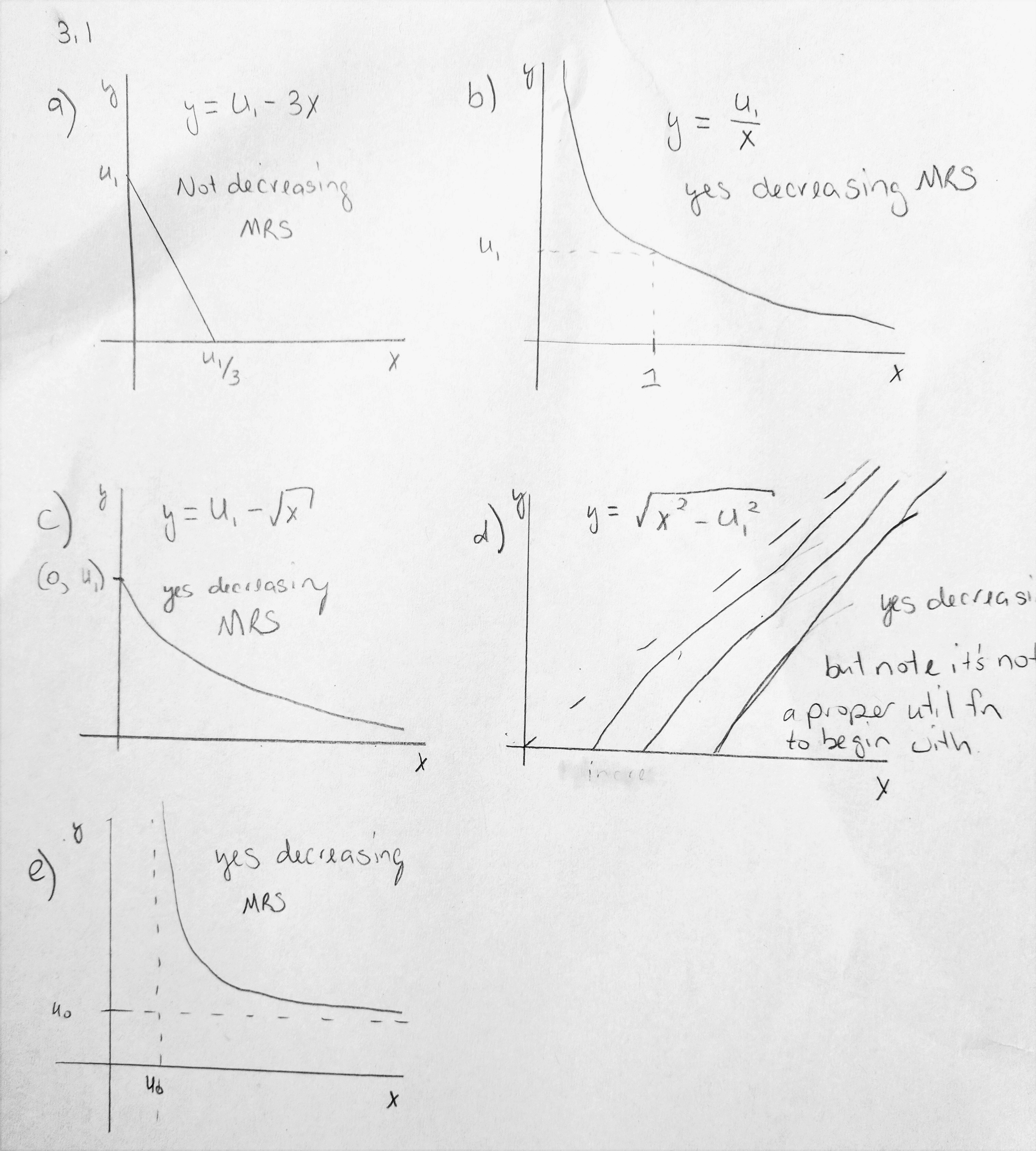
a-e indifference curves

3.3

$U(x,y) = xy$

From above, $MRS = \frac{U_1}{x^2}$ and we verified it was decreasing MRS.

Marginal Utilities:

\[\frac{\partial U}{\partial x} = y\]

which is constant with respect to $x$.

\[\frac{\partial U}{\partial y} = x\]

which is constant with respect to $y$.

$U(x,y) = x^2y^2$

Similarly, $MRS = \frac{\sqrt{U_1}}{x^2}$, which we showed was decreasing.

Marginal Utilities:

\[\frac{\partial U}{\partial x} = 2xy^2\]

which is increasing in x.

\[\frac{\partial U}{\partial y} = 2x^2y\]

which is increasing with respect to $y$.

$U(x,y) = ln(x) + ln(y)$

Show that $y = \frac{e^{U_1}}{x}$ is the equation for a general indifference curve and $MRS = \frac{e^{U_1}}{x^2}$, and show that it is decreasing.

Marginal Utilities:

\[\frac{\partial U}{\partial x} = \frac{1}{x}\]

and

\[\frac{\partial U}{\partial y} = \frac{1}{y}\]

both marginal utilities are increasing.

What can we conclude from this??

We can conclude that decreasing marginal utility is not necessary to get diminishing $MRS$ and quasi-concavity.

The book makes a bid deal out of this, because, in the U.S. it is common to teach the intuition for decreasing $MRS$ by starting with decreasing marginal utility. And it makes a very good intuitive explanation of how utility math functions can be related to actual human behavior, but mathematically, it is not technically required to have decreasing marginal utility to get decreasing $MRS$.

3.5

perfect compliments
1 hot dog perfectly fixed with condiments
$1 + 0.25 + 0.05 + 0.30 = \$1.60$
$cost = \$2.10$ a percent increase of $31\%$
$cost = \$1.725$ lower percent increase ($7.8\%$) because the bun is a smaller component of the overall cost.
Spread the tax so there is no waste of utility. A hot dog with all the condiments only needs to cost $\$2.60$ a $62.5\%$ increase. Thus increase the cost of each component by $62.5\%$.

\[1.625(1*\$1 + 0.5*\$0.50 + 1*\$0.05 + 2*\$0.15) = \$2.60\]

3.7

At point $(6,5)$ the $MRS = \frac{1}{3}$ and
at point $(12,3)$ the $MRS = \frac{1}{3}$

This can only happen with a linear indifference curve. Find the equation by finding the line through the two points. Using the point-slope form of a line from algebra, we find the indifference curve through $(6,5)$ can be expressed as:

\[7 = y + \frac{1}{3}x\]

Then, 7 takes the place of our utility level we usually call $U_1$, and we can write the general utility function as:

\[U(x,y) = y + \frac{1}{3}x\]

The problem description implies that $MRS = \frac{1}{4}$. Further, we know the $MRS$ of a Cobb-Douglass utility function is given by:

\[MRS = \frac{\alpha}{1-\alpha} \frac{y}{x}\]

Then, by plugging in the $MRS$ value and the point, we can recover $\alpha$.

\[\begin{align*} \frac{1}{4} & = \frac{\alpha}{1-\alpha} \frac{1}{8} \\ \alpha & = (1-\alpha)2 \\ \alpha & = \frac{2}{3} \\ 1-\alpha & = \frac{1}{3} \end{align*}\]

and so now we know the full utility function.

3.10

Does not depend on $\alpha + \beta = 1$. To see this, suppose $\alpha + \beta \neq 1$. Then since preferences are indifferent to a monotonic transformation, substitute $\alpha = \frac{\alpha}{\alpha + \beta}$ now $\alpha + \beta = 1$ (go ahead and check it!).
If $y=x$ then $MRS=\frac{\alpha}{\beta}$ so if $\alpha>\beta$ then $MRS>1$.

Intuition: The relative size of $\alpha$ to $\beta$ says the extent to which you prefer $x$ to $y$.

$MRS = \frac{\alpha}{\beta}\frac{(y-_0)}{(x-x_0)}$. Not homothetic since you can’t express as ratio of $x$ to $y$.

3.13

$MRS = \left. \frac{1}{\frac{1}{y}} \right|_{U = constant} = y$

or using another method, set $y=e^{-x+U_1}$, where $U_1$ is an arbitrary constant. Then, $MRS = -[-e^{-x +U_1}]=e^{-x+U_1} = y$.

With this utility function depends only on the level of $y$, whereas usually the bundle containing $x$ and $y$ contributes to the MRS. Sometimes $x$ is called the numeraire good, the economic entity that serves as the standard by which value is computed in an economy. All other goods’ value can be expressed in terms of how much of the numeraire it required to trade for the good. Intuitive examples are gold or fiat money, but any economy that has a good that functions like currency functions like a numeraire.

Wikipedia article - Quasilinear Utility

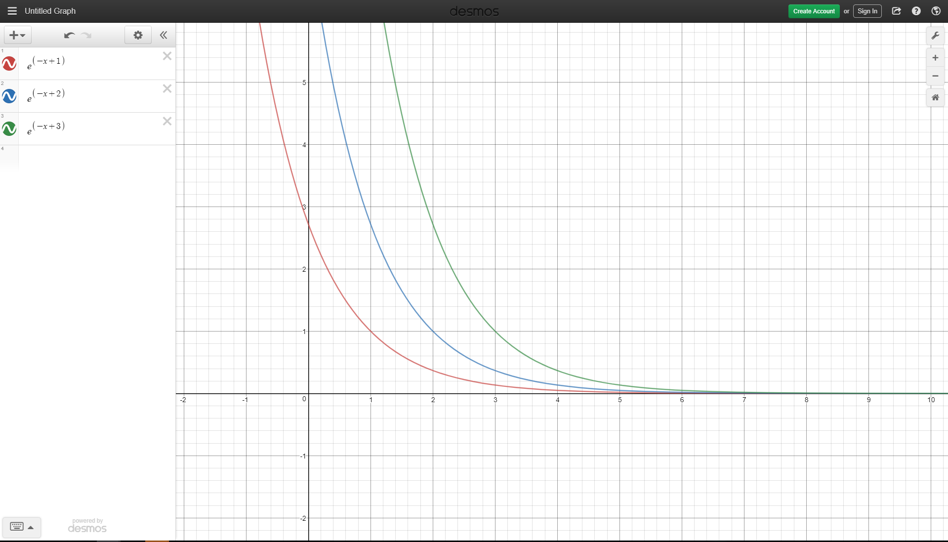
This figure uses the desmos.com calculator to show several indifference curves setting $U_1 = 1, 2, \text{ and } 3$ respectively.

Now adding tangent lines to each indifference curve when $y=1$.

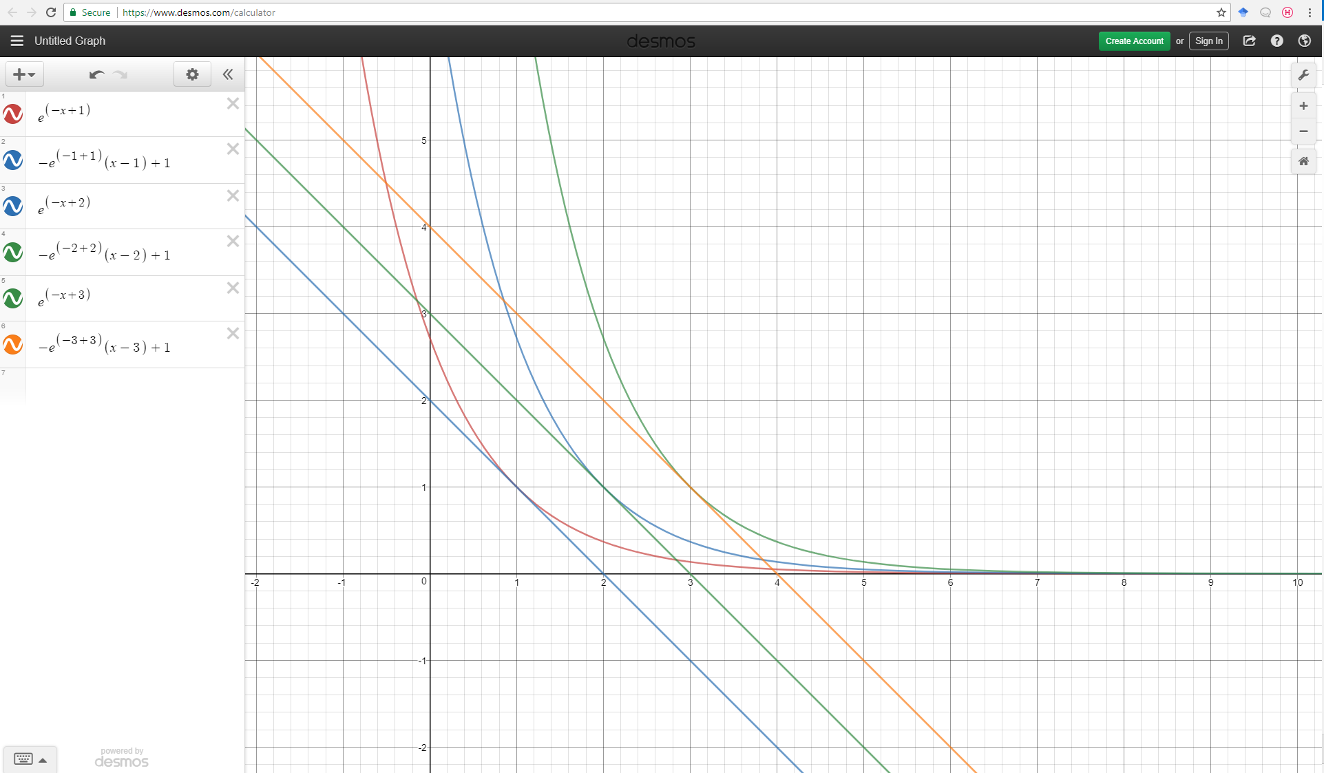
The tangent lines when $y=1$ are clearly parallel, so the MRS is constant when $y=1$. This illustrates that the MRS depends only on y and not on the x value.

Imagine now that the tangent lines are budget lines, then you can see that as income increases, only the consumption of x increases. The consumption of good y is not subject to a wealth effect. All income effects are captured by the numeraire, x.

Note from a that the MRS is decreasing in $x$ (y is after all a function of x…), so the function is quasi-concave.
$y=e^{-x+U_1}$, where $U_1$ is an arbitrary constant.
$\frac{\partial U}{\partial x} = 1$ and
$\frac{\partial U}{\partial y} = \frac{1}{y}$

Notice that the marginal utility of $x$ is constant, so as you buy more, the marginal utility of x is not diminishing.

The question here is trying to lead you toward discovering the concept of a numeraire good.

Desmos Graphin Calculator Demo