Chapter 10 Solutions

Contributed by Noé Nava and Brant Bruxvoort 2017

The following function exhibits economies of scope: \[C(q_1,0)+C(0,q_2)>C(q_1,q_2)\] 10.2

The above inequality exhibits a production function of a firm producing two different goods at a lower cost than two firms producing each good separately. This inequality captures the concept of efficiency: Even though two firms could produce each good separately at the lowest cost of production possible for them, the multi-product firm is able to achieve lower costs than them at the same level of efficiency.
We know that the average costs fall as quantity increases, and that the average cost of a firm producing one good is greater than the average cost of a multi-product firm producing the same good. The expressions below capture this, \[\frac{C(q_1)}{q_1}>\frac{C(q_1+q_2)}{q_1+q_2}\] and \[\frac{C(q_2)}{q_2}>\frac{C(q_1+q_2)}{q_1+q_2}\] If we multiply each inequality by $q_1$and $q_2$, respectively, we obtain, \[q_1(\frac{C(q_1)}{q_1})>q_1(\frac{C(q_1+q_2)}{q_1+q_2})\] and \[q_2(\frac{C(q_2)}{q_2})>q_2(\frac{C(q_1+q_2)}{q_1+q_2})\]

Next, we combine both inequalities adding the left hand side terms and the right left hand side, maintaining the sign as follows, \[q_1(\frac{C(q_1)}{q_1})+q_2(\frac{C(q_2)}{q_2})>q_1(\frac{C(q_1+q_2)}{q_1+q_2})+q_2(\frac{C(q_1+q_2)}{q_1+q_2})\] Notice that we can re-write the above expression to get, \[q_1(\frac{C(q_1)}{q_1})+q_2(\frac{C(q_2)}{q_2})>(q_1+q_2)(\frac{C(q_1+q_2)}{q_1+q_2})\] Finally, we can simplify the expression as follows, \[C(q_1)+C(q_2)>C(q_1+q_2)\] Therefore, we know that this multi-product firm enjoys economies of scope.

10.3 The following equation represents the production function of Professor Smith and Professor Jones: \[q=S^.5*J^.5\] a) To obtain the number of hours that Professor Jones needs to spend to produce a finish book of $q$ number of pages, we have to solve the above equality for $J$. \[q=S^.5*J^.5\] \[\frac{q}{S^.5}=J^.5\] \[J=\frac{q^2}{S}\] Next, we plug in the value for $S$ \[J=\frac{q^2}{900}\] Finally, we plug in the values of $q$ we want to analyze ($q$ = 150, 300 and 450): \[J=\frac{150^2}{900}=25\] \[J=\frac{300^2}{900}=100\] \[J=\frac{450^2}{900}=225\]

To obtain the cost of production, we will sum the cost for Professor Smith’s time with the cost of Professor Jone’s time as follows, \[C(q)=3*(900)+\frac{12}{900}q^2\] The first term is the cost of Professor Smith’s time, and the second term is the cost of Professor Jone’s time. Next, we calculate the Marginal Cost, \[MC(q)=\frac{24}{900}q\] Finally, we plug in the values of $q$ we want to analyze ($q$ = 150, 300 and 450): \[MC(q)=\frac{24}{900}*150=4\] \[MC(q)=\frac{24}{900}*300=8\] \[MC(q)=\frac{24}{900}*450=12\]

10.4 The firm’s fixed proportion production function is given by, \[q=min(5k,10l)\] a) First, notice that a firm experiencing a proportion production finds efficiency whenever it produces at a certain rate of inputs given by, \[5k=10l\] The above ratio means that the firm produces efficiently whenever it uses twice as much productive capital as labor; you can solve by $k$ and $l$ to verify. Next, we calculate the quantity the firm produces at the level of efficiency, \[q*=5k\] and \[q*=10l\] Where $q*$ denotes quantity at the level of efficiency. Since we are analyzing the amount of inputs, we solve the above two equalities by $k$ and $l$ to get, \[k*=\frac{q}{5}\] and \[l*=\frac{q}{10}\] Where $k*$ and $l*$ denote productive capital and labor at the level of efficiency. Next, we calculate the firm’s long run Total Cost, $LTC$, Average Cost, $LAC$ and Marginal Cost, $LMC$. The form of this firm’s $LTC$ operating at the level of efficiency is: \[LTC=vk*+wl*\] Where $v$ is the cost for each unit of productive capital, $k$, and $w$ is the wage of each unit of labor, $l$. Finally, we plug in the values for $k*$ and $l*$, and calculate $LAC$ and $LMC$: \[LTC=v\frac{q}{5}+w\frac{q}{10}\] \[LAC=\frac{v}{5}+\frac{w}{10}\] \[LMC=\frac{v}{5}+\frac{w}{10}\] b) We know that in the short run $k$ must be constant since the firm cannot liquidate or buy more productive capital. Using part a information, we know that if $k=10$, the firm will produce $q=50$, and $l=5$. Notice that these inputs will guarantee efficiency. Finally, the firm’s short run Total Cost, $STC$, Average Cost, $SAC$ and $SMC$ are given by, \[STC=10v+w\frac{q}{10}\] \[SAC=10\frac{v}{q}+\frac{w}{10}\] \[SMC=\frac{w}{10}\] c) If $v=1$ and $w=3$ the firm’s long run Total Cost, $LTC$, Average Cost, $LAC$ and Marginal Cost, $LMC$. The form of this firm’s $LTC$ operating at the level of efficiency is: \[LTC=\frac{1}{5}q+\frac{3}{10}q\] \[LAC=\frac{1}{2}\] \[LMC=\frac{1}{2}\]

10.5

$q=2\sqrt{kl}$
$k=100$ in short run $v=1$ $w=4$

a) Calculate short run total cost. \[ \begin{align} \mathscr{L}&=1(100)+4l+\lambda [q-2\sqrt{l(100)}]\ \\ \mathscr{L}&=100+4l+\lambda [q-20\sqrt{l}] \end{align} \]

FOC: $4-\lambda 10l^{-1/2}=0$ $q=20\sqrt{l}$ $\Rightarrow (\frac{q}{20})^2=l^*$ Short run total cost $\Rightarrow$ $SC(v, w, q)=100+4\frac{q^2}{400}$ $SAC=\frac{100}{q}+\frac{q}{100}$ $SMC=(100+\frac{q^2}{100})=\frac{q}{50}$

b) c) d) Also see figure. $SAC=\frac{100}{q}+\frac{q}{100}$ $SMC=\frac{q}{50}$ $\frac{100}{q}+\frac{q}{100}=\frac{q}{50}$ $\frac{100}{q}=\frac{2q-q}{100}$ $\frac{100}{q}={q}{100}$ $100=\frac{q^2}{100}$ $100=q$ (this is also min of SAC)

e) $q=2\sqrt{\bar{k}l}$ $(\frac{q}{2\sqrt{\bar{k}}})=l^c$

$SC(v, w, q, k=\bar{k})=v\bar{k}+w(\frac{q^2}{4k})$

f) Minimize short run costs over $\bar{k}$ $ _ {{k}}SC(v, w, q, k={k})$

\[\begin{align} \frac{\mathrm{d}}{\mathrm{d} \bar{k}}(v\bar{k}+w\frac{q^2}{4\bar{k}})&=\frac{\mathrm{d}}{\mathrm{d} \bar{k}}(v\bar{k}+\frac{w}{4}\bar{k}^{-1} q^2)\\ &=v-\frac{wq^2}{4\bar{k}^2}=0\\ \end{align}\]

Solve for $\bar{k}$

\[ \begin{align} v&=\frac{wq^2}{4\bar{k}^2}\\ 4v\bar{k}^2&=wq^2\\ \bar{k}^2&=\frac{wq^2}{4v}\\ \bar{k}&=\sqrt{\frac{w}{v}}\frac{q}{2}\\ \end{align} \]

since both must be positive (note typo in book solution here)

g) If $k$ is calculated correctly in (f) then plugging cost minimizing $\bar{k}$ into $SC$ should give us the long run cost function.

\[ \begin{align} SC(v, w, q, \bar{k}&=\sqrt{\frac{w}{v}}\frac{q}{2})=v[\sqrt{\frac{w}\\{v}}\frac{q}{2}]+w[\frac{q^2}{4}[\sqrt{\frac{w}{v}}\frac{q}{2}]]\\ &=\sqrt{v}\sqrt{w}\frac{q}{2}+\sqrt{v}\sqrt{w}\frac{q}{2}\\ &=\sqrt{v}\sqrt{w}q\\ &=c(v, w, q) \end{align} \]

This is the long run cost function for Cobb-Douglas

h) See figure.

The long run cost curve is an ‘envelope’ of the short run cost curves.

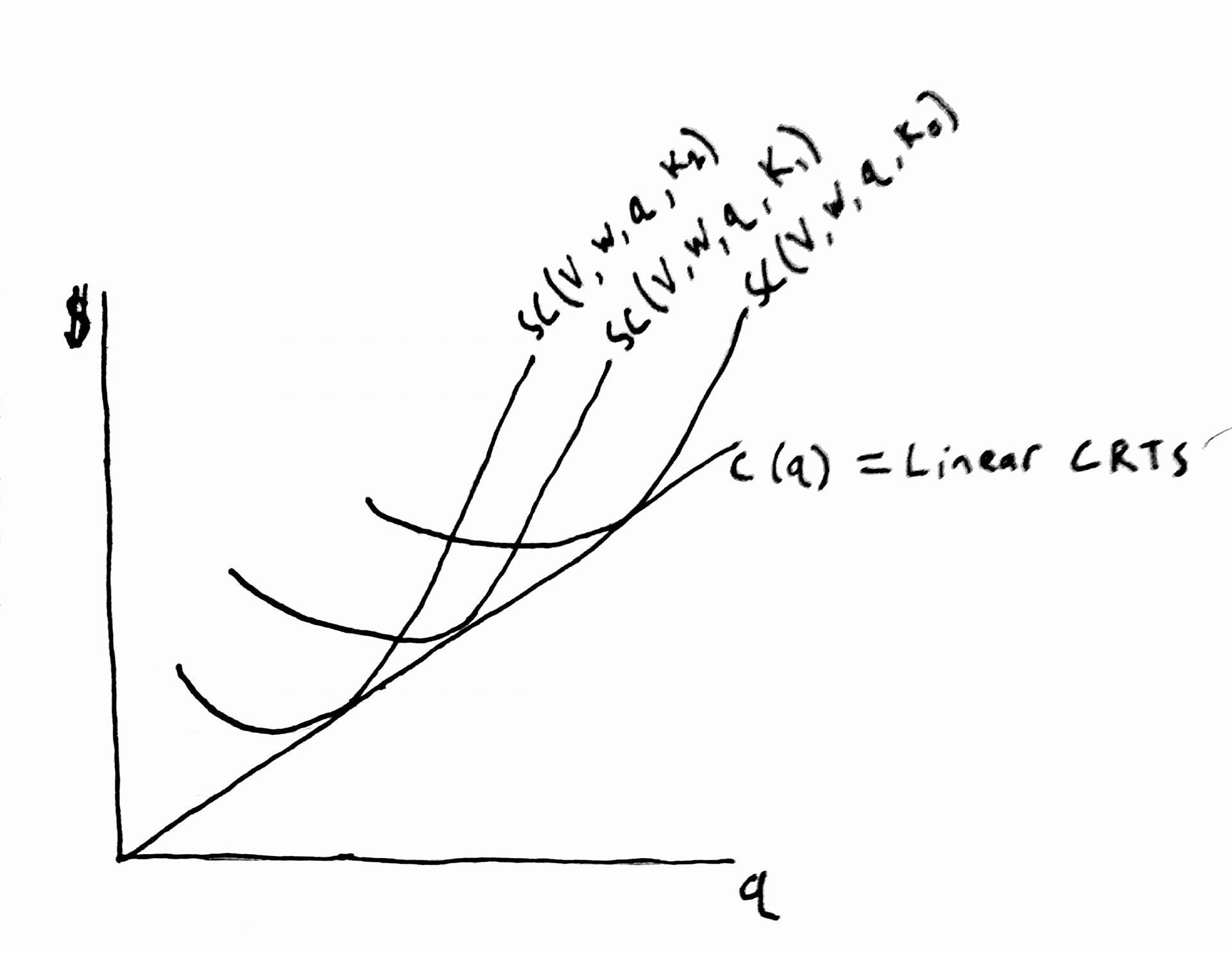
Figure for 10.5 b,c, and d

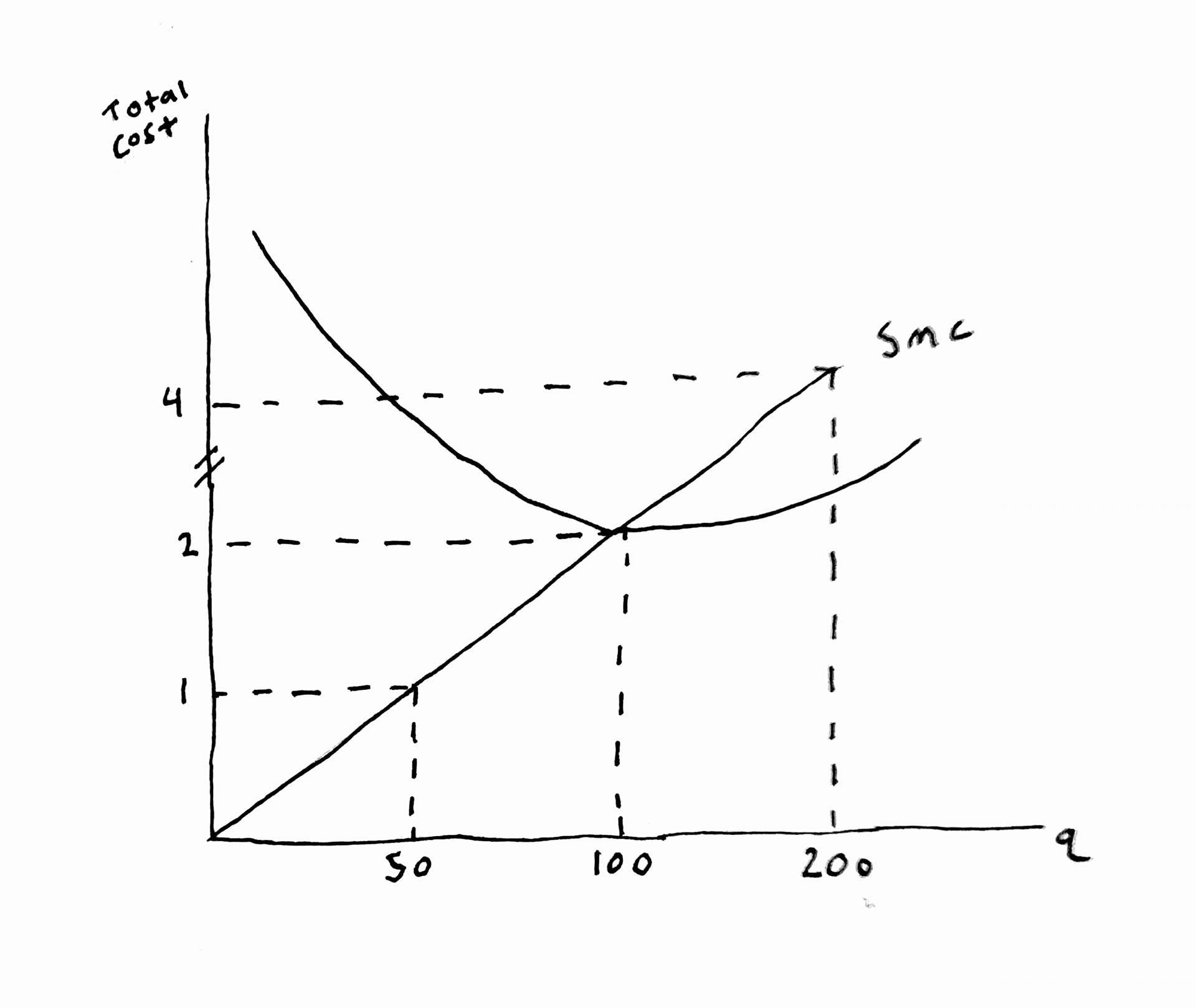
Figure for 10.7 h

10.7

$l^*=\frac{\partial{c}}{\partial{w}}=\frac{2}{3}qw^{-1/ 3}v^{1/3}$ $k^*=\frac{\partial{c}}{\partial{v}}=\frac{1}{3}qw^{2/ 3}v^{-2/3}$

b) Both equations above have $(\frac{v}{w})$ in them.

$l^*=\frac{2}{3}q(\frac{v}{w})^{1/3}$

$l^*=\frac{1}{3}q(\frac{v}{w})^{-2/3}$

Solve for $(\frac{v}{w})$ in each, then set equal to each other.

\[ \begin{align} [\frac{l^*\frac{3}{2}}{q}]^3&=\frac{v}{w}\\ [\frac{k^*(3)}{q}]^{-3/2}]&=\frac{v}{w}\\ [\frac{l\frac{3}{2}}{q}]^3&=[\frac{k(3)}{q}]^{-3/2}]\\ \end{align} \]

This is a relationship between $q$ & $k$ & $l$…a production function! Solve for q.

\[ \begin{align} \frac{(\frac{3l}{2})^3}{q^3}&=\frac{(3k)^{-3/2}}{q^{-3/2}}\\ (\frac{3l}{2})^3(3k)^{-3/2}&=q^3\cdot q^{3/2}\\ 3^3(\frac{1}{2})^33^{3/2}l^3k^{3/2}&=q^{9/2}\\ 3^{9/2}(\frac{1}{2})^3l^3k^{3/2}&=q^{9/2}\\ 3(\frac{1}{2})^{2/3}l^{2/3}k^{1/3}&=q\\ 3(\frac{1}{4})^{1/3}l^{2/3}k^{1/3}&=q\\ \end{align} \] This looks more like a production function!

10.8

$c=q(v+s\sqrt{vw}+w)$

\[ \begin{align} &k^* = \frac{\partial c}{\partial v}=q+v^{-1/2}w^{1/2}q \Rightarrow k=q+(\frac{v}{w})^{-1/2}\cdot q\\ &l^*=\frac{\partial c}{\partial w}=q+v^{1/2}w^{-1/2}q \Rightarrow l=q+(\frac{v}{w})^{1/2}\cdot q \end{align} \]

\[ \begin{align} &\frac{k}{q}=1+(\frac{v}{w})^{-1/2} & &\frac{l}{q}=1+(\frac{v}{w})^{1/2}\\ &[\frac{k}{q}-1]^{-2}=\frac{v}{w} & &[\frac{l}{q}-1]^2=\frac{v}{w}\\ \end{align} \]

\[ \begin{align} [\frac{k}{q}-1]^{-2}&=[\frac{l}{q}-1]^2\\ \frac{1}{\frac{k}{q}-1}&=[\frac{l}{q}-1]\\ \frac{q}{k-q}&=\frac{l-q}{q} \end{align} \]

\[ \begin{align} &q^2-(l-q)(k-q)=0\\ &q^2-[lk-lq-kq+q^2]=0\\ &q(l+k)-lk=0\\ &q=\frac{lk}{l+k} \end{align} \]

CES with $\rho =1$ and note that the book should have told us to assume $\gamma = 1$. Without it, we cannot work out the problem.

\[\begin{align*} C(r,w,q) &= q^{\frac{1}{\gamma}}(r^{1-\sigma} + w^{1-\sigma})^{\frac{1}{1-\sigma}} \\ &= q(r^{0.5} + w^{0.5})^2 \\ &= q(r + 2\sqrt{vw} + w) \end{align*}\]

Which is what we were asked to show.