Chapter 4 Solutions
4.1
- The utility function, \(U(t,s)=\sqrt{ts}\), is really just Cobb-Douglass utility with \(\alpha = 0.5\) and \(\beta = 0.5\), so using the solution we derived in the notes,
\[t^* = \frac{I}{2p_t} \text{ and } s^* = \frac{I}{2p_s}\].
Substituting in for \(I= 1, p_t = 0.10,\) and \(p_s = 0.25\), we find the solution, \(t^* = 5,\) and \(s^* = 2\).
- Indirect utility is useful here.
\[V(p_t, p_s, I) = \frac{I}{2p_t^{0.5}p_s^{0.5}}\]
Increase income by \(k\) to achieve same utility level. To find, we solve for \(k\) in the following equation,
\[V(0.40, 0.25, 1+k) = V(0.10, 0.25, 1)\],
or in plain English, solve for \(k\) such that the utility achieved under the new prices and additional income is the same as the utility achieved with the old prices and income.
Solve:
\[\begin{align*} \frac{1+k}{2*0.40^{0.5}*0.25^{0.5}} &= \frac{1}{2*0.10^{0.5}*0.25^{0.5}} \\ k &= \frac{0.40^{0.5}*0.25^{0.5}}{0.10^{0.5}*0.25^{0.5}} - 1 \\ k &= $1 \end{align*}\]His mother should send $2, a $1 increase.
4.2
- \(w_F^* = \frac{\alpha}{\alpha + \beta} \frac{I}{p_F}\), and \(w_C^* = \frac{\beta}{\alpha + \beta} \frac{I}{p_C}\)
Substitute in the parameters given in the problem.
\[\begin{align*} w_F^* &= \frac{2}{3} \frac{600}{40} \\ &= 10 \end{align*}\] \[\begin{align*} w_C^* &= \frac{1}{3} \frac{600}{8} \\ &= 25 \end{align*}\]- California wine purchased stays the same, but now French wine purchased is,
Because the French wine is now cheaper she can buy more for the same income and achieve higher utility. To put a monetary value on it, check how much she would be willing to reduce her income in order to face the new (lower) prices.
\[V(20, 8, 600-k) = V(40, 8, 600)\],
she is willing to reduce income by as much as \(k\) to get the new lower price.
\[\begin{align*} \left( \frac{2}{3} \right) ^{\frac{2}{3}} \left( \frac{1}{3} \right) ^{\frac{1}{3}} \frac{600-k}{20^{\frac{2}{3}}8^{\frac{1}{3}}} &= \left( \frac{2}{3} \right) ^{\frac{2}{3}} \left( \frac{1}{3} \right) \frac{600}{40^{\frac{2}{3}}8^{\frac{1}{3}}} \end{align*}\]solving for \(k\)
\[\begin{align*} 600 - k &= \frac{600*20^{\frac{2}{3}}8^{\frac{1}{3}}}{40^{\frac{2}{3}}8^{\frac{1}{3}}} \\ k &= 600 - \frac{600}{2^{\frac{2}{3}}} \\ k &= 222.02 \end{align*}\]An alternative monetary measure would be to check how much she would be willing to accept (increase income) to keep the old prices. This is equivalent to the concepts if equivalent variation and compensating variation that are presented in chapter 5.
4.3
In this problem his consumption of \(c\) and \(b\) is constrained so that \(c+b = 5\). We can use a Lagrangian function to solve the constrained optimization problem.
\[\mathscr{L} = 20c - c^2 + 18b - b^2 + \lambda[5-c-b]\]
The first order conditions of the Lagrangian problem are:
\[\begin{align*} 20 - 2c - \lambda &= 0 \\ 18 - 6b - \lambda &= 0 \\ 5 -c -b &= 0 \end{align*}\]solving for \(b\) and \(c\) gives \(b = 1\) and \(c = 4\).
4.4
- Maximising \(U(x+y)= x^2+y^2\) won’t alter the results because MRS is unchanged under a monotonit increasing transformation.
\[\mathscr{L} = x^2 + y^2 +\lambda[50-3x-4y]\]
The first order conditions of the Lagrangian problem are:
\[\begin{align*} 2x - 3\lambda &= 0 \\ 2y - 4\lambda &= 0 \\ 50 - 3x - 4y & = 0 \end{align*}\] Combining eqns 1 and 2, \(\frac{x}{y} = \frac{3}{4}\). Substituting in to equation 3, the budget line, we get:\[\begin{align*} 50 &= 3 \left( \frac{3}{4}y \right) + 4y \\ 50 &= \frac{9y}{4} + 4y \\ 50 &= \frac{25y}{4} \\ \end{align*}\]
So, \(y = 8\) and \(x = 6\).
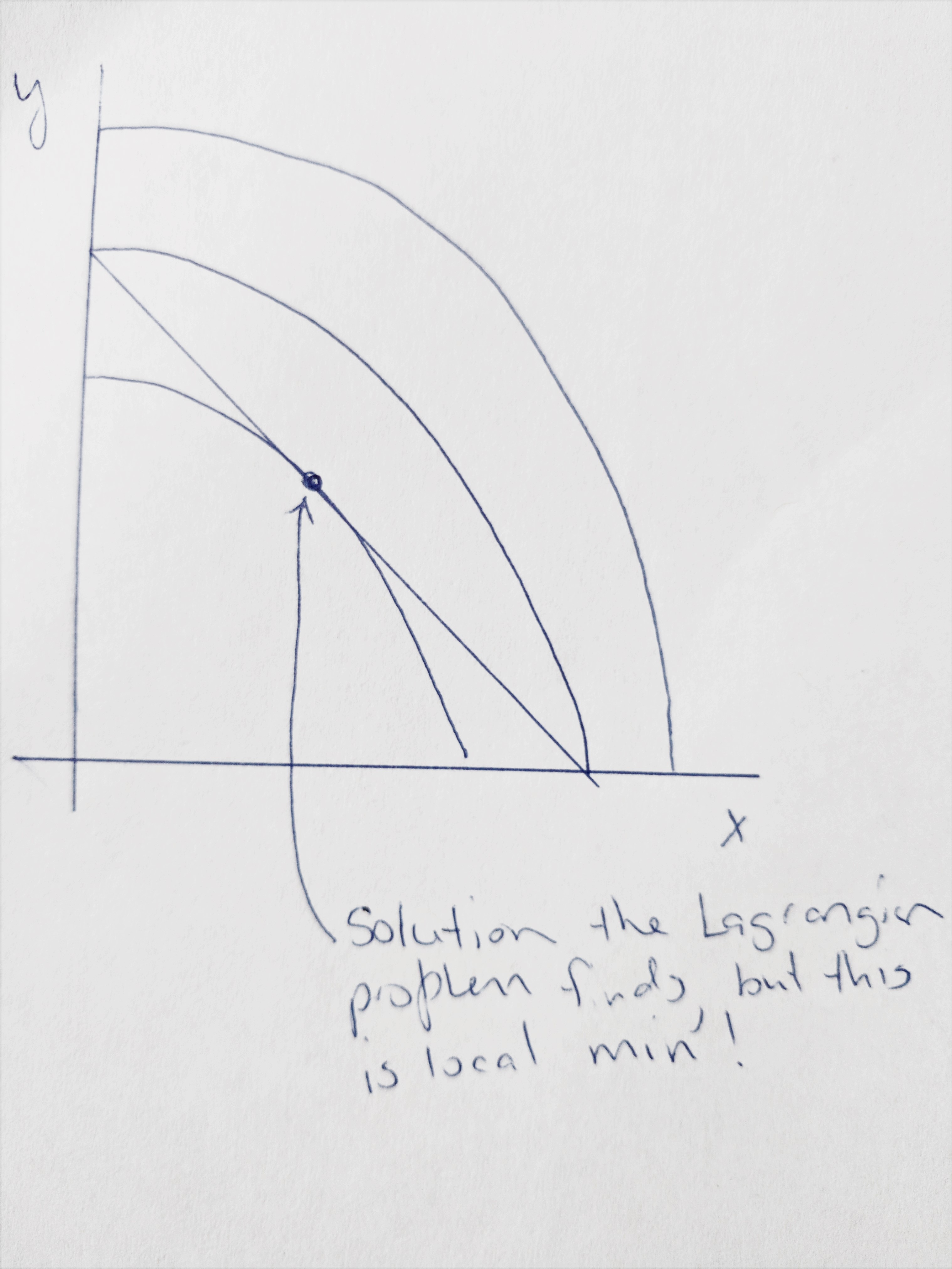
Since the indifference curves are not convex, the solution to the problem is actually a local minimum, not a local maximum!
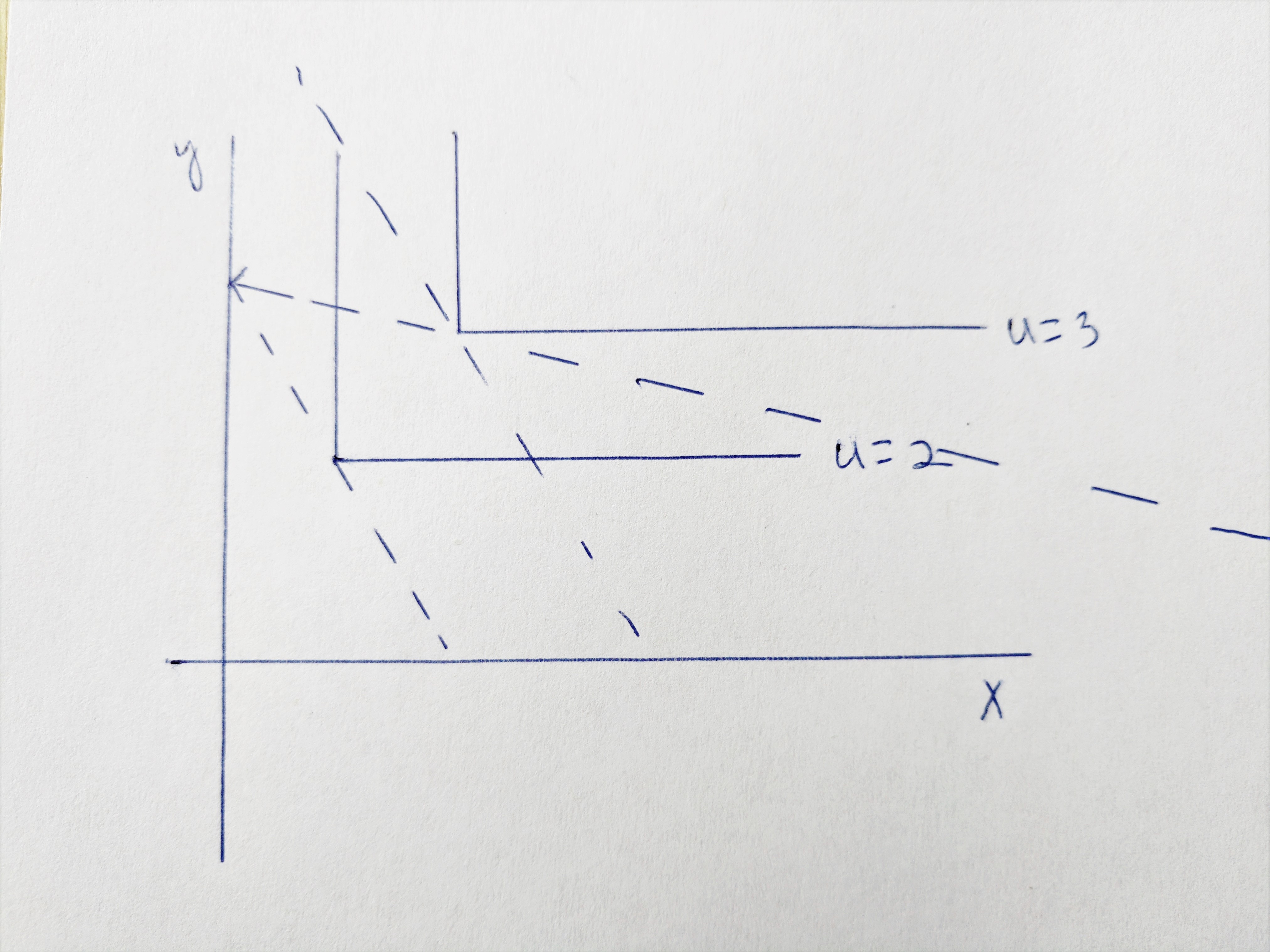
4.7.
This graph is in our lecture notes.
The expenditure required to achieve utility of 2.
The expenditure required to achieve utility of 3.
\[\begin{align*} e(p_x, p_y, U) &= 2p_x^{\frac{1}{2}}p_y^{\frac{1}{2}}U \\ e(1, 4, 2) &= 2*1^{\frac{1}{2}}*4^{\frac{1}{2}}2 \text{ using example 4.4 prices}\\ &= \$8 \end{align*}\] \[\begin{align*} e(1, 4, 3) &= 2*1^{\frac{1}{2}}*4^{\frac{1}{2}}3 \text{ using example 4.4 prices}\\ &= \$12 \end{align*}\]So it is $4 extra (\(\$4 = \$12 - \$8\))
- Assuming the same expenditureof $8, how much would we have to subsidise \(x\) to achieve utility of 3? Solve the following:
Solving yields \(s = \$\frac{5}{9}\). To calculate the cost to the government, multiply by the quantity of x purchased.
\[\frac{5}{9}x^* = \frac{5}{9}\frac{8}{2(1-\frac{5}{9})} = \$5\]
If the objective is to raise utility from 2 to 3, it is cheaper for the government to give an income grant of $4 than to subsidise the purchase of \(x\), because that would cost $5.
This is the lump sum principle.
- The general expediture function for Cobb-Douglas utility is given by \(e(p_x, p_y, U) = \frac{p_x^{\frac{1}{2}}p_y^{\frac{1}{2}}U}{\alpha^{\alpha} \beta^{\beta}}\), and for \(\alpha = 0.3\), the quantity \(\alpha^{\alpha} \beta^{\beta} \approx 0.543\).
So, achieving utility of 2 requires
\[e(1, 4, 2) = \frac{1^{0.3}*4^{0.7}2}{0.543} = 9.774\]
while achieving utility of 3 requires
\[e(1, 4, 2) = \frac{1^{0.3}*4^{0.7}3}{0.543} = 14.66\]
which is $4.89 extra.
- Because there are no substitution effects in the fixed proportion case, the optimal point would be the same and also the cost to govt would be same.
4.10
- The solution to a utility max problem with \(U(x,y) = x^{\alpha}y^{1-\alpha}\) is
\[x^* = \alpha\frac{I}{p_x} \text{ and } y^* = \beta\frac{I}{p_y}\]
Then indirect utility is\[\begin{align*} V(p_x,p_y, I) &= \left[ \alpha\frac{I}{p_x} \right]^{\alpha} \left[ \beta\frac{I}{p_y} \right]^{\beta} \\ &= \alpha^{\alpha}(1-\alpha)^{\alpha}\frac{I}{p_x^{\alpha}*p_y^{\beta}} \end{align*}\]
- Since the indirect utility function is right in front of us, we can use duality to derive the expenditure function from the indirect utility function.
Since income is equal to expenditure, we replace \(I\) with \(e(p_x,p_y,\overline U)\), and replace \(V(p_x,p_y, I)\) with \(\overline U\).
\[\overline U = \alpha^{\alpha}(1-\alpha)^{\alpha}\frac{e(p_x,p_y,\overline U)}{p_x^{\alpha}*p_y^{1- \alpha}} \]
Now, solving for \(e(p_x,p_y, U)\)
\[e(p_x,p_y, U) = \frac{p_x^{\alpha}*p_y^{1- \alpha}* \overline U}{\alpha^{\alpha}(1-\alpha)^{\alpha}} \]
The compensation required to offset the effect of a price rise of \(x\) can be expressed as
\[\begin{align*} e(p_x^1,p_y, \overline U) - e(p_x^0,p_y, \overline U) = \frac{\left(p_x^1\right)^{\alpha}*p_y^{1- \alpha}* \overline U}{\alpha^{\alpha}(1-\alpha)^{\alpha}} - \frac{\left(p_x^0\right)^{\alpha}*p_y^{1- \alpha}* \overline U}{\alpha^{\alpha}(1-\alpha)^{\alpha}} \end{align*}\]This expression obviously varies with \(\alpha\) and the higher the \(\alpha\) the more compensation needed. One could attempt to differentiate this expression with respect to \(\alpha\) but that would be a yucky derivative so we’ll skip it.