Chapter 5 Solutions
Contributed by Samantha Forrest 2017
5.1Ed can purchase water in a 0.75 liter and 2 liter bottle. He regards the two goods as perfect substitutes.
a.) Assuming Ed’s utility depends on the quantity of water consumed, express the utility function in terms of quantities of 0.75L containers (x) and 2L containers (y).
\[x=\frac{3}{4}L\] \[L=\frac{4}{3}x\]
so, \[\frac{y}{2}=\frac{4}{3}x\]
\[\frac{3}{8}y=x\] so, \[u= x+ \frac{3}{8}y\]That is that x little bottles contributes the same to utility as 3/8 of a big bottle.
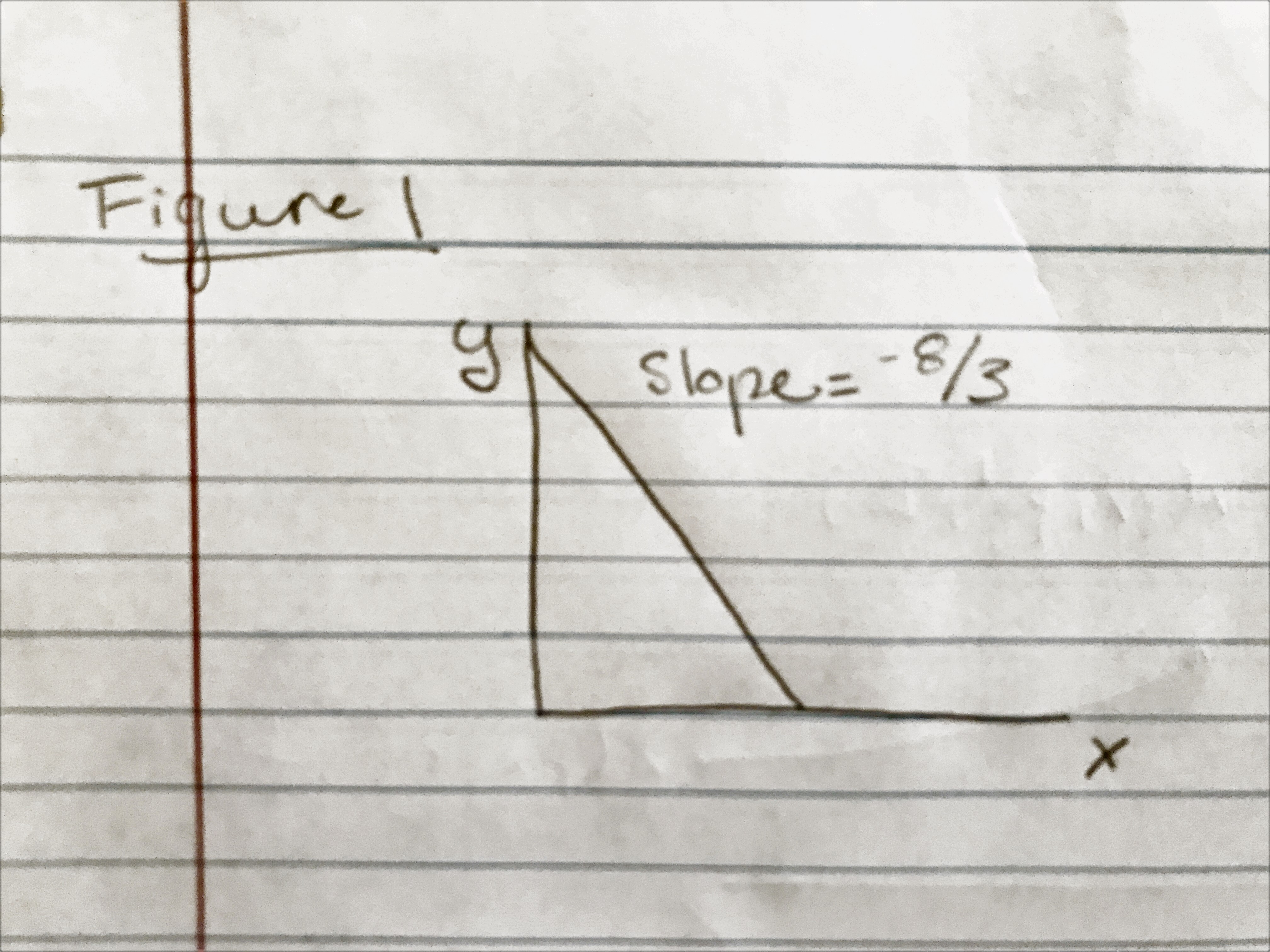
Figure 1
b.) State Ed’s demand function for x in terms of \(p_x, p_y,\) and I.
\(x=\frac{I}{p_x}\) if \(p_x\leq\frac{8}{3}p_y\)If the price of the little bottle is less than \(\frac{8}{3}\) the price of the big bottle, he should buy all little bottles.
c.) Graph the demand curve for x, holding I and p_y constant.
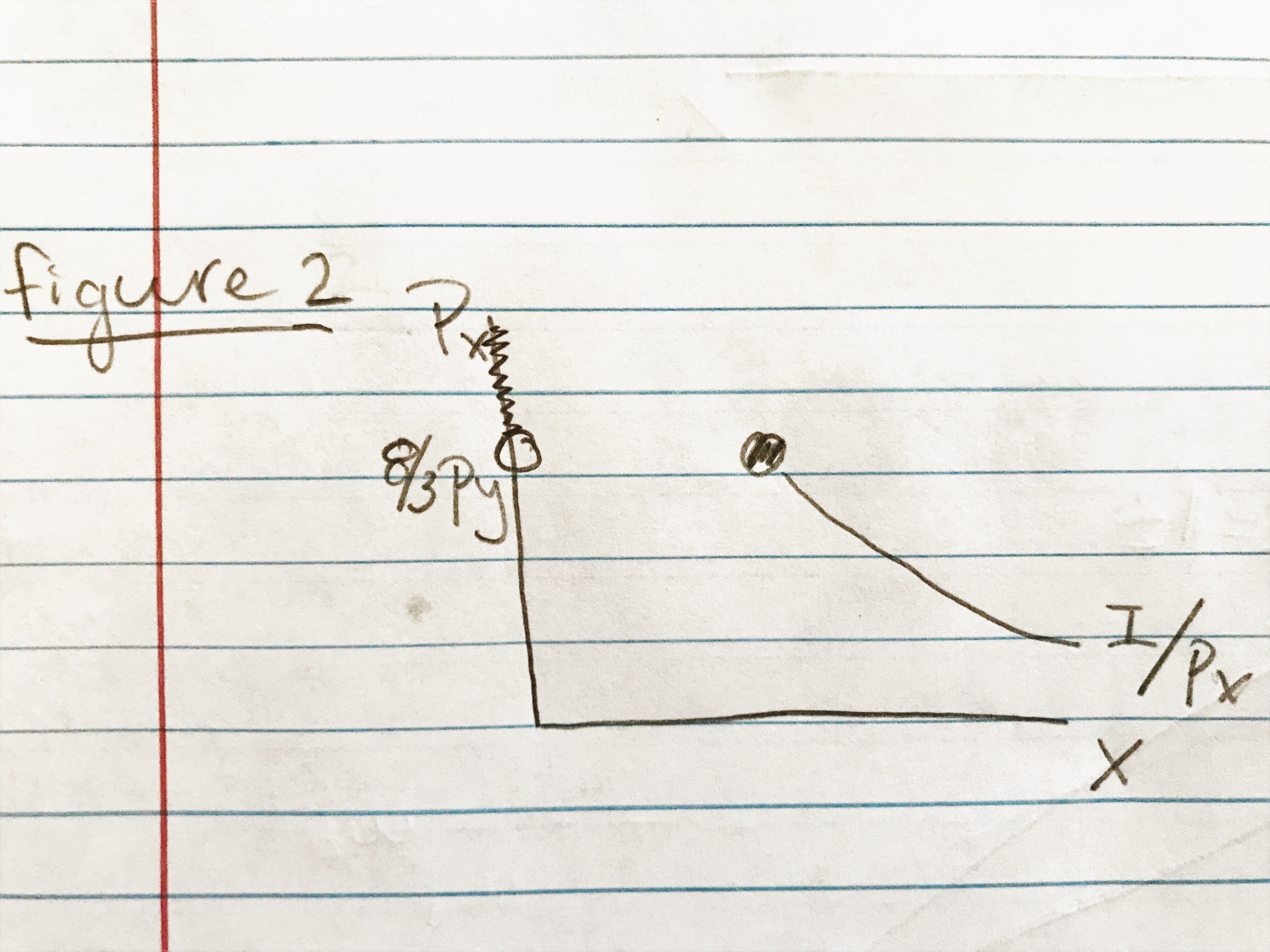
Figure 2
d.) How do changes in I and \(p_y\) shift the demand curve for x?
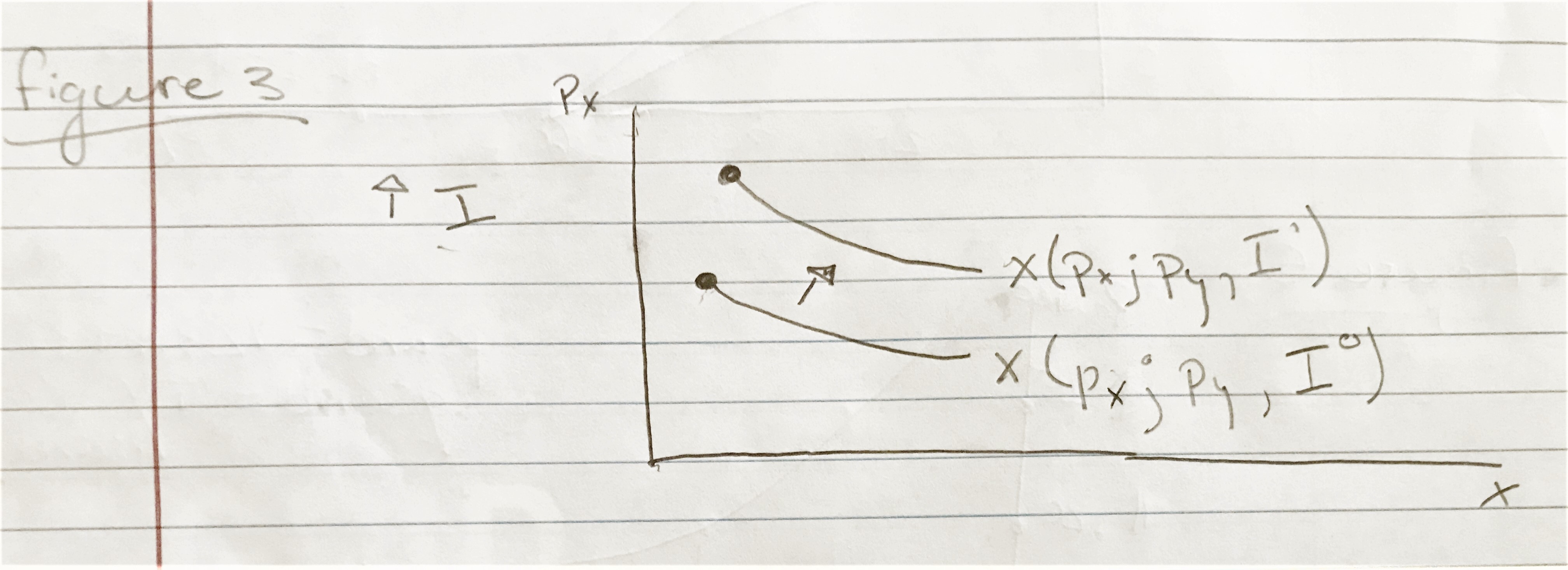
Figure 3a
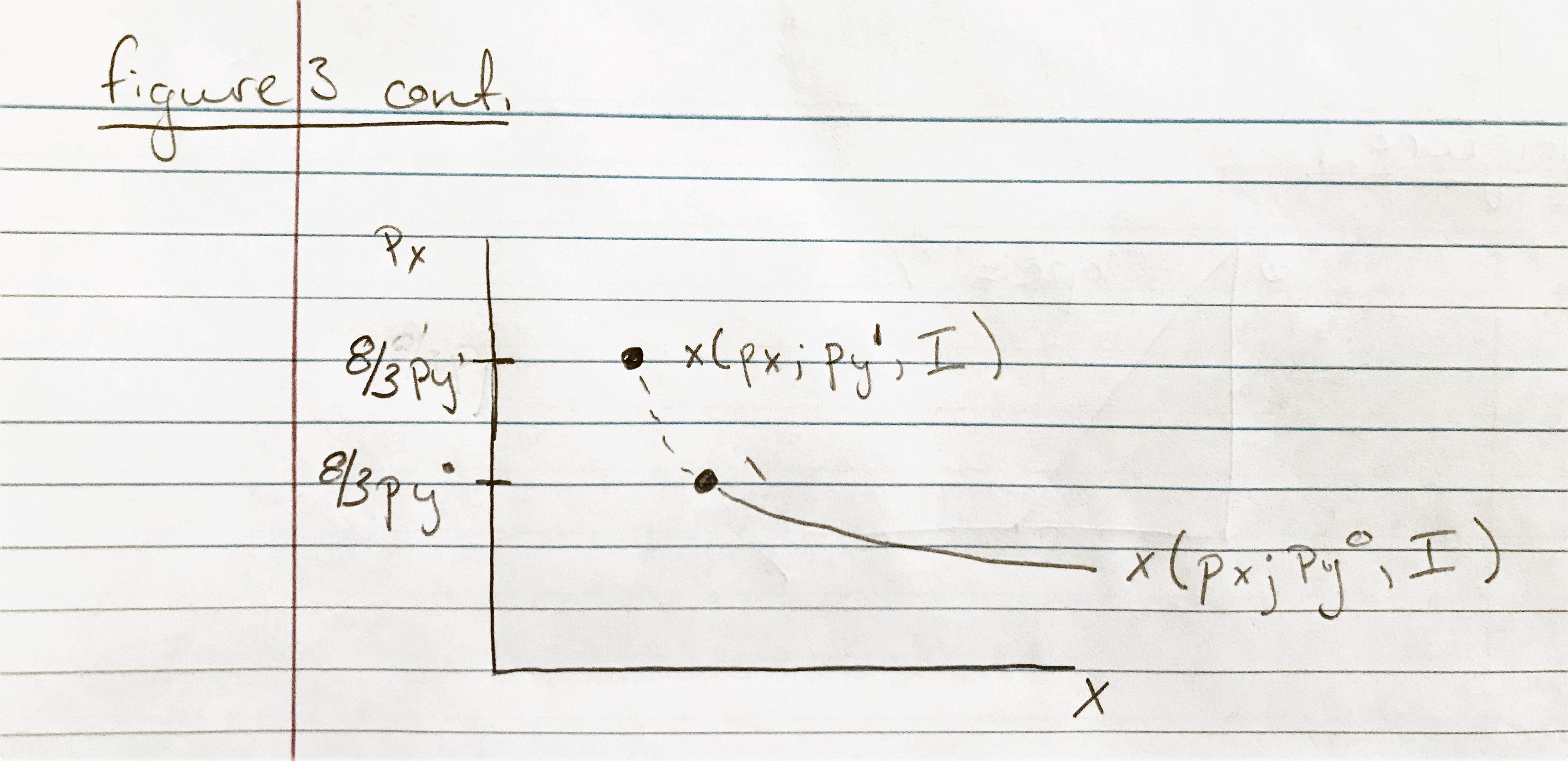
Figure 3b
David receives only $3 a week and cares only about a particular sandwich bundle that is peanut butter and jelly. He uses exactly 1 oz of jelly and 2 oz of peanut butter for each sandwich.
a.) How much peanut butter and jelly will David buy with his $3 allowance in a week?
\[$Sandwhich=.05\times{2} + .1\times{1}\] \[=.1+.1\] \[=$.20\] \[\frac{$3}{$.20}=15 sandwiches\]
Davide will buy 15 oz jelly and 30 oz peanut butter in a week.
b.) Suppose the price of jelly were to rise to $0.15 an oz. How much of each commodity will be bought?
\[$Sandwich=.05\times2+.15\times1\] \[=$.25\] \[\frac{$3}{$.25}= 12 Sandwiches\]
David will buy 12 oz of jelly and 24 oz of peanut butter.
c.) By how much should David’s allowance be increased to compensate for the rise in price in jelly in part (b)?
\[15\times.25=$3.75\]
He needs $0.75 in compensation to be able to eat 15 sandwiches again.
d.) Graph your results in parts (a) to (c).
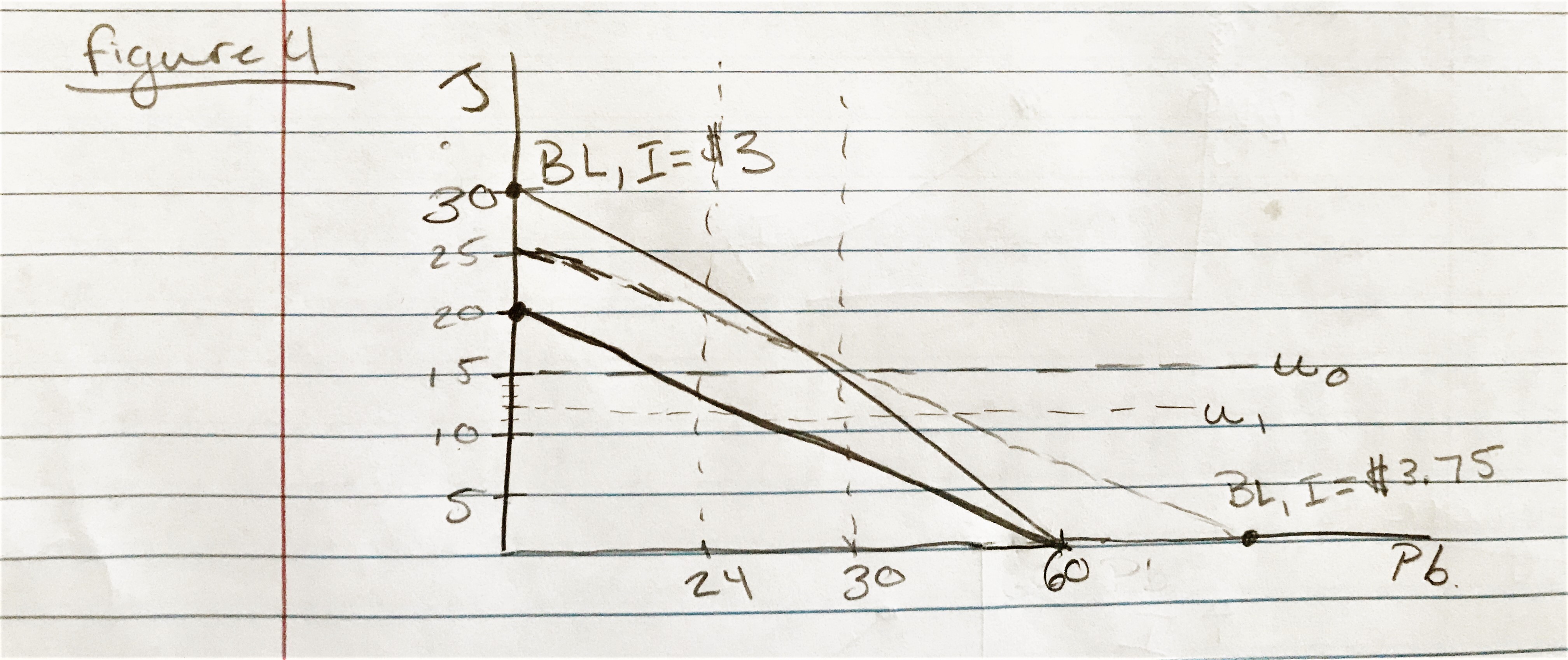
Figure 4
- In what sense does this problem involve only a single commodity: peanut butter and jelly sandwiches? Graph the demand curve for this single commodity.
Since he really is interested in sandwiches, the components are consumed in fixed proportions.
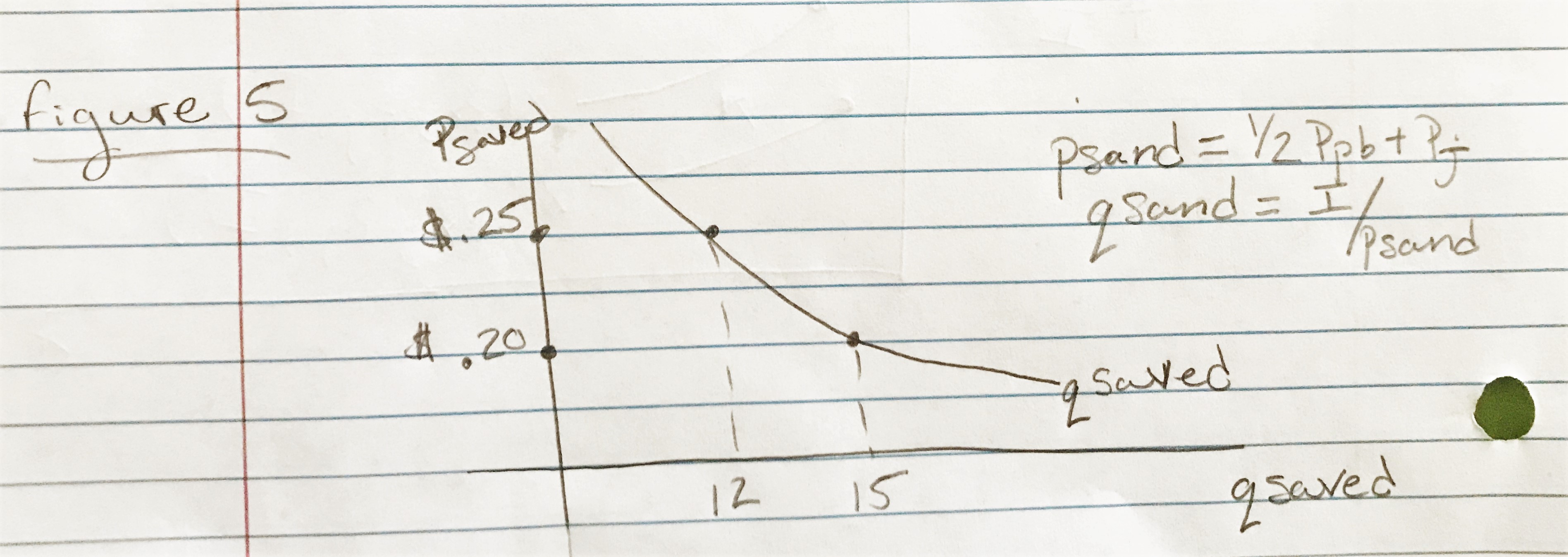
Figure 5
f.) Discuss the results of this problem in terms of the income and substitution effects involved in the demand for jelly.
No substitution effect. It is all manifest through the income effect.
5.5
Suppose the utility function for goods x and y is given by \(utility=U(x,y)=x\cdot{y}+y\).
a.)Calculate the uncompensated (Marshallian) demand function for x and y and describe how the demand curves for x and y are shifted by changes in I or the price of the other goods.
\[U(x,y)=x\cdot{y}+y\] \[!!!=x\cdot{y}+y+\lambda[I-p_x-p_y]\] FOC:
\[y-\lambda\cdot{p_x}=0\] \[x+1-\lambda\cdot{p_y}=0\] \[ \Rightarrow \frac{y}{x+1}=\frac{p_x}{p_y} \Rightarrow y=\frac{p_x}{p_y}\cdot{(x+1)}\] \[I=p_x\cdot{x}+p_y\cdot{y} \Rightarrow I=p_x\cdot{x}+p_x\cdot{(x+1)} \Rightarrow \frac{I-p_x}{2p_x}=x^\star\] \[y^\star=\frac{p_x}{p_y}\cdot{\frac{I-p_x}{2p_x}}=\frac{1}{2p_y}[I+p]\]An increase in income increase consumption of both x & y, but a price increase in x decrease consumption of x & increases consumption of y. An increase in the price of y decreases only consumption of y.
b.) Calculate the expenditure function for x and y.
\[V(p_x,p_y,I)= \frac{I-p_x}{2p_x}\cdot{\frac{I+p_x}{2p_y}}+\frac{I+p_x}{2p_y}\] \[\bar{u}=\frac{I+p_x}{2p_y}\cdot{\frac{I+p_x}{2p_x}}\] \[\sqrt{4p_xp_y\bar{u}}-p_x=I\] \[e(p_x,p_y,\bar{u})=2\sqrt{p_xp_y\frac{1}{u}}-p_x\]
c.) Use the expenditure function calculated in part (b) to compute the compensated demand functions for goods x and y. Describe how the compensated demand curves for x and y are shifted by changes in income or by changes in the price of the other good.
Two Ways:
1.) Plug e in for I in the Marshallian demands
\[x^c(p_x,p_y,\bar{u})=\frac{2\sqrt{p_xp_y\frac{1}{u}}-2p_x}{2p_x}=\frac{\sqrt{p_y\bar{u}}-\sqrt{p_x}}{\sqrt{p_x}}\] \[y^c(p_x,p_y,u)=\frac{2\sqrt{p_xp_y\bar{u}}}{2p_y}=\frac{\sqrt{p_x\bar{u}}}{\sqrt{p_y}}\]
2.) Shephard’s Lemma (p.167)
\[x^c(p_x,p_y,\bar{u})=\frac{\partial{e(p_x,p_y,\bar{u})}}{\partial{p_x}}\] \[=\frac{\sqrt{p_y\bar{u}}}{\sqrt{p_x}}-1=\frac{\sqrt{p_y\bar{u}}-\sqrt{p_x}}{\sqrt{p_x}}\] \[y^c(p_x,p_y,\bar{u})=\frac{\partial{p_x,p_y,\bar{u}}}{\partial{p_y}}\]\[=\frac{\sqrt{p_x\bar{u}}}{\sqrt{p_y}}\]
The compensated demand curves are unaffected by changes in income. They do, however, show that both cross prices affect x & y.
5.10 More on elasticities
Part (e) of Problem 5.9 has a number of useful applications because it shows how price responses depend ultimately on the underlying parameters of the utility function. Specifically, use that result together with the Slutsky equation in elasticity terms to show:
a.) In the Cobb-Douglas case (\(\sigma=1\)), the following relationship holds between the own-price elasticities of \(x\) and \(y: e_{x,p_x}+e_{y,p_y}=-2\).
First, Slutsky equation in elasticities
Remember, \(\frac{\partial{e}}{\partial{p_x}}=x^\star(p_x,p_y,\bar{u})\)
\[\frac{\partial{x^\star}}{\partial{p_x}}=\frac{\partial{x^c}}{\partial{p_x}}-\frac{\partial{x^\star}}{\partial{e}}\cdot{\frac{\partial{e}}{\partial{p_x}}}\] \[\frac{\partial{x^\star}}{\partial{p_x}}=\frac{\partial{x^c}}{\partial{p_x}}-\frac{\partial{x^\star}}{\partial{e}}\cdot{x^c}\]multiply through by \(\frac{p_x}{x}\)
\[\frac{\partial{x^\star}}{\partial{p_x}}\cdot{\frac{p_x}{x}}=\frac{\partial{x^c}}{\partial{p_x}}\cdot{\frac{p_x}{x}}-\frac{\partial{x^\star}}{\partial{e}}\cdot{x^c}\cdot{\frac{p_x}{x}}\]
multiply by \(\frac{e}{e}=1\) in income term
\[e_{x,p_x}=e^c_{x,p_x}-\frac{\partial{x^\star}}{\partial{e}}\cdot{\frac{e}{e}}\cdot{\frac{p_xx^c}{x}}\]
Substitute\(\frac{\partial{x^\star}}{\partial{e}}\cdot{\frac{e}{x}}=e_{x,I}\)
\[e_{x,p_x}=e^c_{x,p_x}-e_{x,I}\cdot{\frac{p_xx^c}{e}}\]
Substitute \(e=I\).
\[e_{x,p_x}=e^c_{x,p_x}-e_{x, I}\cdot{\frac{p_xx^c}{I}}\]
Substitute \(s_x=\) share of income spent on x.
\[e_{x,p_x}=e^c_{x,p_x}-e_{x, I}\cdot{s_x}\]
Now using 5.9 (e) \(e^c_{x,p_x}=-(1-s_x)\sigma=-(1-s_x)\) in the Cobb Douglass Case.
\[e_{x,p_x}=-(1-s_x)-e_x,I^{s_x}\]
Since \(e_{x,I}=1\) in Cobb Douglass case.
\[e_{x,p_x}=-1\]
Similarly for y, then \(e_{x,p_x}+e_{y,p_y}=-2\). Similarly you can show that \(e_{y,p_y}=-1\Rightarrow{e_{x,p_x}+e_{y,p_y}=-2}\)
b.) If \(\sigma>1\) then \(e_{x,p_x}+e_{y,p_y}<-2\), and if \(\sigma<1\) then \(e_{x,p_x}+e_{y,p_y}>-2\). Provide an intuitive explanation for this result.
Again by the slutsky equation in elasticities.
\[e_{x,p_x}=e^c_{x,p_x}-e_{x,I}\cdot{s_x}\] \[e_{x,p_x}= -(1-s_x)\sigma-e_{x,I}\cdot{s_x}\]
Since CES is homothetic, \(e_{x,I}=1\)
\[e_{x,p_x}=-(1-s_x)\sigma-s_x\] \[e_{x,p_x}=-\sigma+\sigma{s_x}-s_x\]\[=-\sigma+s_x(\sigma-1)\]
Similarly for y: \(e_{y,p_y}=-\sigma+s_y(\sigma-1)\)
\[\Rightarrow{e_{x,p_x}+e_{y,p_y}=-2\sigma+s_x(\sigma-1)+s_y(\sigma-1)}\] \[=-2\sigma-[s_x+s_y]+\sigma[s_x+s_y]\] \[-2\sigma-1+\sigma\] \[=-\sigma-1\]
\(<-2\) when \(\sigma>1\)
\(>-2\) when \(\sigma<1\)
Intuition
Written with StackEdit.