23 Appendix: Single Market Models: ARIMA
Interested in more? Please let me know by taking the survey!
In this chapter we introduce the first category of time-series econometric forecasting models we will learn: Auto-regressive Integrated Moving Average (ARIMA) models. This class of models is only capable of forecasting one market at a time, and we will see in later chapters how to econometrically consider (forecast) more than one market at a time when there is reason to believe two or markets are related.
The ARIMA class of models can be broken down into subcategories that are useful for building intuition.
23.1 Integrated or Not?
We spent considerable effort in Chapters 10 and 11 on the importance of stationarity in estimating time-series forecasting models. If a series is stationary it is said to be ‘Integrated of Order Zero’, or I(0), or not integrated; if a series is non-stationary, but the first (log) difference of the series is stationary then the series is said to be ‘Integrated of Order One’, or I(1); if a series is non-stationary, but the second (log) difference of the series is stationary then the series is said to be ‘Integrated of Order Two’, or I(2); and so forth. The number of times required to difference the data before it becomes stationary determines the order of integration. As discussed in Chapter 11, it is a relatively safe assumption that our price data will be integrated of order one, and thus first (log) differences of the data should be used.
With all that said, the ‘I’ in ARIMA stands for integrated, and simply signifies the functional forms that follow can be implemented with price levels (no differencing) if the data are stationary and in differences if the data are non-stationary. We will always use first differenced data for the examples in this class.
23.2 \(AR(p)\), Models
In Chapter 10 we introduced the Efficient Market Hypothesis (EMH) that states all information about an asset should be reflected in its current price, and therefore is unpredictable. In Chapter 11, we argued that if the EMH is true than prices should follow a log-normal price model fairly well. Indeed, it is true that a log-normal price model is difficult to beat, or that coming up with an informative forecast is difficult, but there are some common properties of data that can inform a forecasting model.
The first is that recent (changes in) prices can effect the next period’s price realization. Simply put, prices often exhibit auto-correlation in returns. If so, adding lags of price changes in our forecasting model can help to improve forecasts.
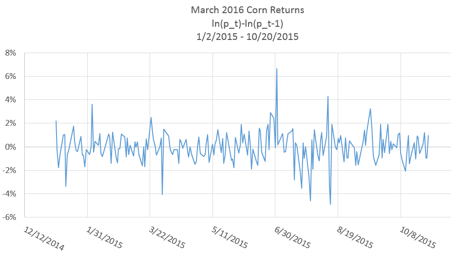
In figure 1 percent returns of the March 2016 corn futures contract are plotted.
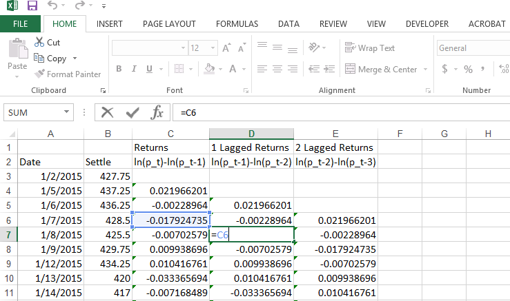
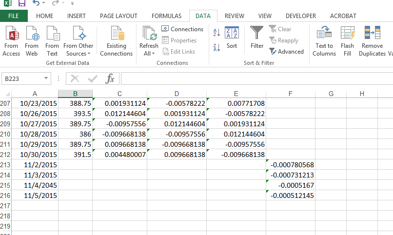
To investigate if a price series exhibits auto-correlation, we need to generate time lags in the price series. Figure 2 shows a screenshot in Excel of how to generate time lags of returns. Basically, you just point the cell to the value in the previous period. Note that the value in D7 simply takes the value in C6.
Now, to get a rough idea if there is auto-correlation in corn returns, we calculate the correlation of columns C, D, and E. This function can be performed in the ‘Data Analysis’ choice of the ‘Data’ menu tab in Excel. The output is displayed in Figure 3.
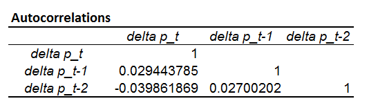
Given the low values of correlations between the contemporaneous price and the one-lag and two-lagged prices, I am not hopeful for the prospects of a good forecast from the \(AR(p)\) model, but we will go ahead and estimate it nonetheless for illustrative purposes.
23.2.1 The \(AR(p)\) Model
The \(AR(p)\) model is formally defined by equation 1.
- \(R_{t+1} = \beta_0 + \beta_1R_{t} + \beta_2R_{t-1}+ ... + \beta_{p}R_{t-(p-1)} + \epsilon_t\)
where \(R_i\) represents the percentage return on period \(i\). The \(p\) in \(AR(p)\) is the number of lagged returns included in the model. In figure 4, we show regression output in Excel from estimating an \(AR(2)\) price model on corn price returns in the March 2016 contract from 1/2/2015 - 10/20/2015.
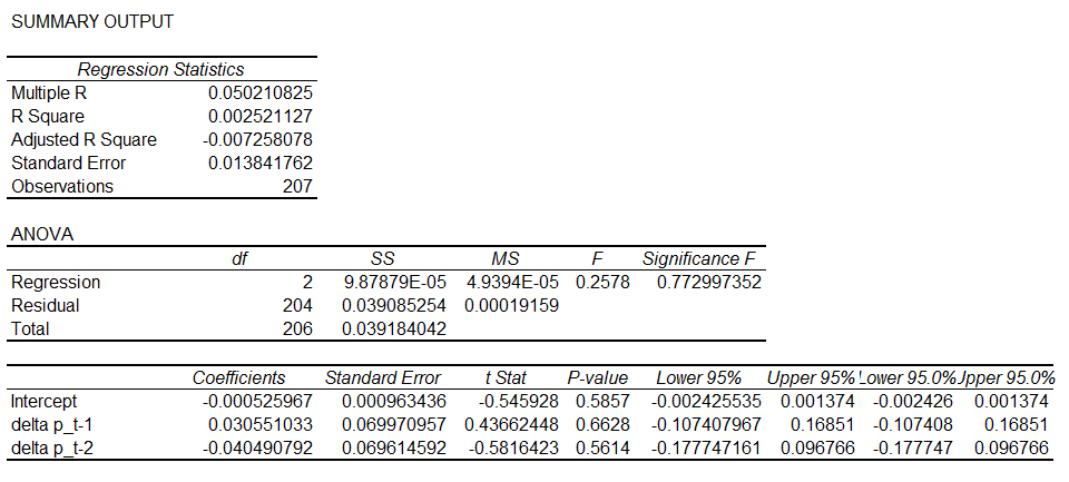
All of the p-values for our regressors are large, certainly much bigger than 0.05. We fail to reject the null hypothesis that one and two lags of corn price returns are unrelated to the next price return realization. Therefore, the \(AR(2)\) model does not seem to provide much forecasting power.
23.3 \(MA(q)\), Models
The Moving Average Model incorporates lagged random shocks into the forecast model. Commonly denoted by \(MA(q)\), the \(q\) stands for the number of lags of shocks to be included. Formally,
- \(R_{t+1} = \theta_0 + \epsilon_t + \theta_1\epsilon_{t-1} + ... + \theta_q\epsilon_{t-q}\)
Compare this modeling approach with the \(AR(p)\) approach. In the \(AR(p)\) model, lagged shocks incorporated only indirectly through thier effect on lagged returns. In the \(MA(q)\) model, lagged shocks affect current returns directly. Estimating the \(MA(q)\) model is not as simple a metter as estimating the \(AR(p)\) model. We were able to directly estimate the \(AR(p)\) model with ordinary least squares in Excel.
In equation 2, we see that it is impossible to implement with ordinary least squares becasue we need to know the values of the \(\theta_i\) in order to calculate the residuals, \(\epsilon_i\). Instead, we will take an iteritive approach to estimating this model.
23.3.1 Guesing the \(\theta_i\) and Minimising the Sum of Squared Residuals
We discussed in Chapter 11, that linear regression finds estimated coeficients by minimizing the Sum of Squared Residuals. One approach to estimating the $MA(q) model in Excel is to guess the values of the \(\theta_i\) coeficients. That will let us calculate residuals by hand.
- \(\epsilon_{t} = R_{t+1} - (\theta_0 + \theta_1\epsilon_{t-1} + ... + \theta_q\epsilon_{t-q})\)
After that, we can calculate the sum of squared residuals that results from our guess.
- \(\sum_{t=1}^{T} \epsilon_t^2\)
Then we can use the ‘Solver’ function in Excel’s Analysis toolpack to minimize the sum of squared residuals by choosing the \(\theta_i\).
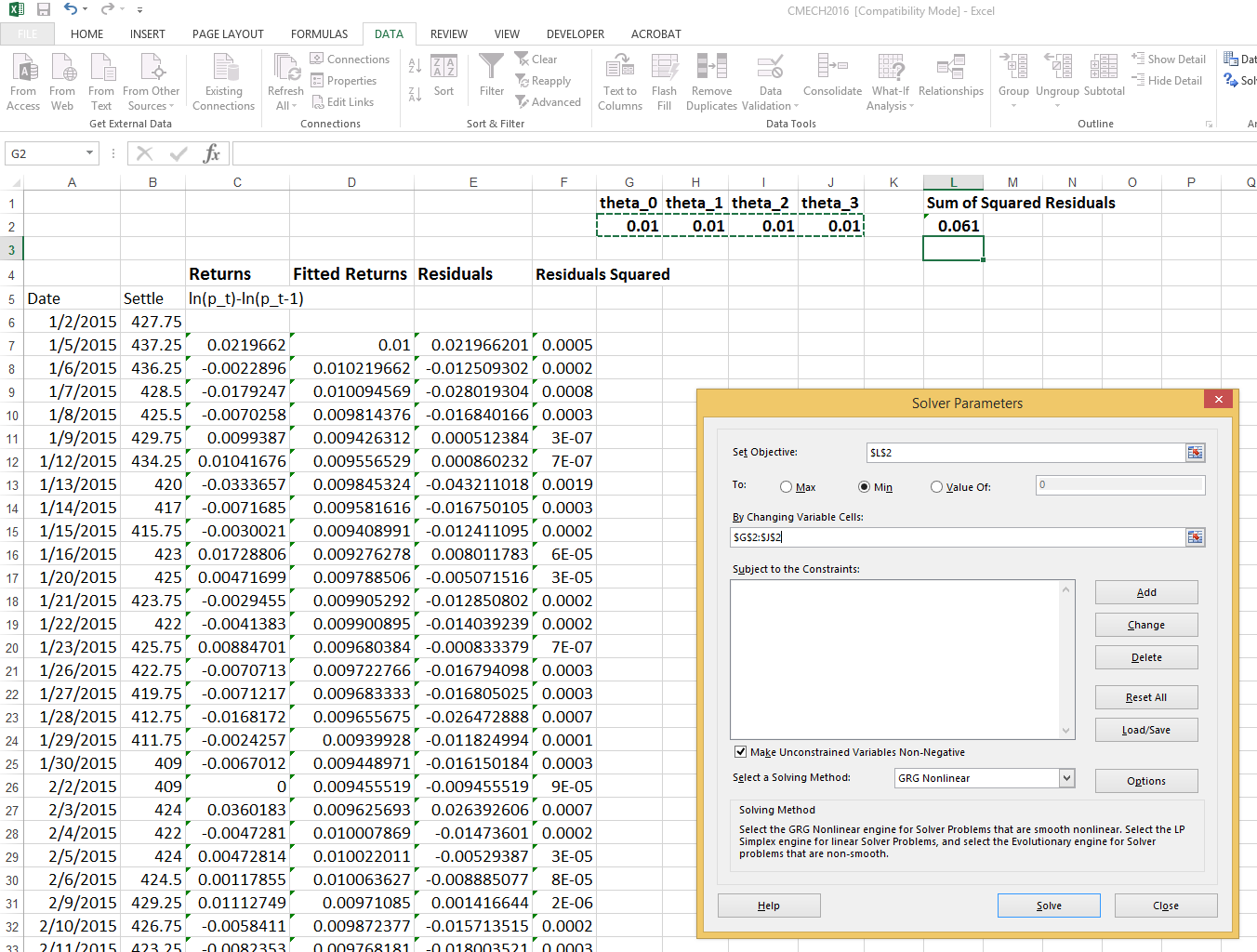
Doing just those steps will give you accurate estimates of the \(\theta_i\) coefficents, but no information of the standard errors of the coefficients so hypothesis testing up this point is not possible. After using the Excel solver functionality to find the \(\theta_i\) that minimizes the sum of squared residuals, you will have accurate calculations of the residuals. You can now regress returns on the calculated residuals to perform hypothesis testing. Your regression coefficients should match the \(\theta_i\) you calculated with the Excel ‘Solver’.

We see that the regression coefficients match very well for \(\theta_0\), \(\theta_1\), and \(\theta_3\), while \(\theta_2\) seems to be off from the calculations we received from the ‘Solver’ function in Excel.
The \(MA(2)\) model does not seem to explain the March 2016 corn returns very well. We are explaining just under 1% of the variation in the data, as shown by the \(R^2\), and none of the coefficients are close to statistical significance since the p-values are all well above 0.05.
23.3.2 Fitting an \(MA(q)\) model in Excel
- Guess \(\theta_i\) values
- Calculate residuals, \(\epsilon_t\)
- Calculate Sum of Squared Residuals
- Use ‘Solver’ to minimize the sum of squared residuals by choosing \(\theta_i\)
- Regress returns on residuals 6 Conduct hypothesis testing
Keep in mind, this process in uneccessarily complicated. If you get seriously involved in generating forecasts, you will invest the time to learn a common statistical package; however, hopefully this process helps to build some intuition about how these models are estimated by the more powerful statistical software packages.
23.4 Lag Length
You may be wondering at this point if it would be useful to try including more lags in the regression equation; perhaps we will find longer lag lengths that seem to matter in forecasting corn price returns. Usually, if lags have predictive power, the strongest effects are in the nearest lags. So adding lags to the \(AR(.)\) model is unlikely to help.
Still, as a practical matter, lag length must be selected before estimating an \(AR(p)\) model. If we were using a more advanced statistical package, we could use Information Criterion1 to select the optimal lag length, but like unit root tests, it is not convenient to implement in Excel so we will not cover Information Criterion.
The intuition of selecting a lag length by Information Criterion is simple enough, though. Basically, a model with a large number of lags is estimated. The longest lags are then sequentially removed one by one, until explanatory power is detrimentally affected by removing a lag. That determines lag length.
As a rough substitute, one could estimate an \(AR(p)\) model for large \(p\). Then sequentially remove the longest lag until the likelihood decreases; or until the F-statistic is dramatically reduced by eliminating lagged variables. In practice, we will be lucky to find any statistically significant coefficients on the lags, and the nearest lags will be most likely to be significant, so a small number of lags will usually be sufficient.
23.5 Dealing with Seasonality
23.6 Caculating Forecast Values
Figure 5 shows a screenshot of Excel where the model output from figure 4 is used to produce the \(AR(2)\) model forecasts shown in column F.
Forecasts are found by using the estimated model and recent realizations of returns to produce a one-step-ahead forecast as follows
- \(\hat{R_{t+1}} = E[\beta_0 + \beta_1R_{t} + \beta_2R_{t-1}+ ... + \beta_{p}R_{t-(p-1)} + \epsilon_t]\)
Since the only random part of the equation is \(\epsilon_t\) and it is iid with mean equal to zero, the one step ahead forecast is found by,
- \(\hat{R_{t+1}} = \beta_0 + \beta_1R_{t} + \beta_2R_{t-1}+ ... + \beta_{p}R_{t-(p-1)}\)
Although we know our forecast model will have an error component, the mean of the error is zero so our forecast simply comes from plugging lags back into our estimated model. Notice the hat on the \(\hat{R_{t+1}}\) that signifies the equation produces a forecast and not an actual realization.
What if we want to gererate a forecast two steps ahead and so forth? Since we do not yet observe \(R_{t+1}\) we use our forecast \(\hat{R_{t+1}}\).
- \(\hat{R_{t+2}} = \beta_0 + \beta_1\hat{R_{t+1}} + \beta_2R_{t}+ ... + \beta_{p}R_{t-(p)}\)
As we produce increasingly distant h-step ahead forecasts, we will run out of realizations and begin plugging in forecasts for the lagged values. Figure 6 Plots the 1-4-step ahead forecasts shown in column F of figure 5, along with the return realizations.
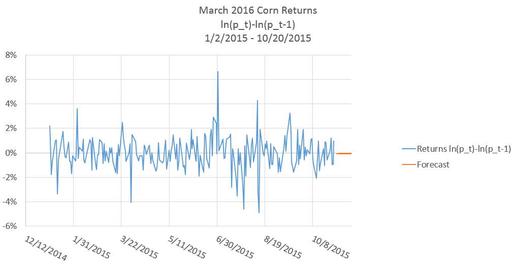
The \(AR(2)\) model more or less forecasts a percent return of zero. This result should be fairly intiutive because we did not find stron autocorrelation in the return series; additionally, the return series itself is roughly mean zero, so the forecast is relying mostly on the unconditional mean (the mean of \(\epsilon\)) because we did not find statistically siginificant autocorrelation coefficients.